Dragan Djuric

• blog https://dragan.rocks
• twitter @draganrocks
• Professor of Software Engineering
• University of Belgrade
• Clojure as a primary language since 2009
• Interested in Bayesian methods in ML.
• [email protected]
• github: blueberry / uncomplicate
• https://uncomplicate.org

A little background

• Clojure
• GPU computing
• Bayesian Data Analysis

Clojure - a modern lisp

• Dynamic and fast
• First-class functions
• Great abstractions and data structures
• Many useful libraries
• Even more experimental libraries
• Seamless access to Java and the JVM
• ClojureScript in browsers, node etc.

Are Java and Clojure good at number crunching?

• Good? maybe.
• Great? NO!
• JVM - no access to hardware-specific optimizations
• We can make it great!

CPU is not so great either!

• R, Python? Even worse than Java.
• C? complicated, verbose platform-specific optimizations.
• CPU? too beefed-up. Burns as the Sun!

GPU has a lot to offer …at a price

• many dumb computing units
• but, power-efficient for number crunching
• hardware support for massive parallelism
• faster and cheaper each year
• notoriously difficult to program

Uncomplicate

Fluokitten

fluorescent monadic fuzzy little things

ClojureCL

take control of the GPU and CPU from Clojure

Neanderthal

optimized vectors and matrices on CPU and GPU

Bayadera

high performance Bayesian statistics and data analysis on the GPU

What does all this has to do with Bayes?

• BDA is conceptually simple
• Real models must be calculated numerically
• MCMC sampling and related methods
• In higher dimensions, requires huge samples
• Analyses typically run in minutes, hours, weeks

.

• Good: Clojure and GPU FTW
• Challenge: MCMC is sequential

A Bayesian Data Analysis Primer

How to know something we cannot observe?

• Probabilities of all answers (prior)
• Probability of measured data (evidence and likelihood)
• Calculate "backwards", using Bayes' rule and get
• posterior probabilities of answers

Doing Bayesian Data Analysis

• John Kruschke
• Excellent tutorial, even for beginners
• Real-world examples through the book!

Hello World: Fair or Trick coin?

• Coin bias, tendency to fall on head: θ
• We can not measure θ directly
• We can only know sample data (D)
• θ is general; θ₁, θ₂, …, θ_n are specific values
• D is general; 3 heads out of 10 specific

By Bayes' rule:

Analytical solution

Likelihood:

Pr(z,N|θ) = θ^z (1 - θ)^N-z

(conjugate) prior

Pr(θ|a,b) = beta(θ|a,b) = θ^(a-1)(1-θ)^(b-1)/B(a,b)

Posterior, conveniently:

Pr(θ|z,N) = beta(θ|z+a, N - z + b)

Example from Kruschke's book

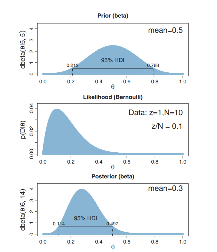
Easy computation

Q: What is Pr(0.4<θ<0.6)?

A: Pr(θ<0.6) - Pr(θ<0.4)

(let [a-prior 5
      b-prior 5
      z 1
      N 10
      a-post (+ a-prior z)
      b-post (+ b-prior (- N z))]

(- (beta-cdf a-post b-post 0.6)
   (beta-cdf a-post b-post 0.4)))

Never happens in practice

• Only the simplest models are "nice"
• The curse of dimensionality

Bayadera

• a Clojure library
  • highly opinionated - Bayesian
  • probabilistic
  • need to NOT be super slow - thus GPU
  • actually is the fastest I have seen
• use cases:
  • Bayesian data analysis (more stats-oriented)
  • a foundation for machine learning algorithms
  • lots of statistical number crunching
  • risk assessment, decision analysis, etc.

Bayadera Goals

• programmers are the first-class citizens
• not a "me too, just in Clojure"
• different and better (for what I want to do)
• for interactive and server use

HARD to compute

Usually:

computationally:

Markov Chain Monte Carlo (MCMC)

• a family of simulation algorithms
• draws samples from unknown probability distributions
• (enough) samples approximate the distribution

computationally:

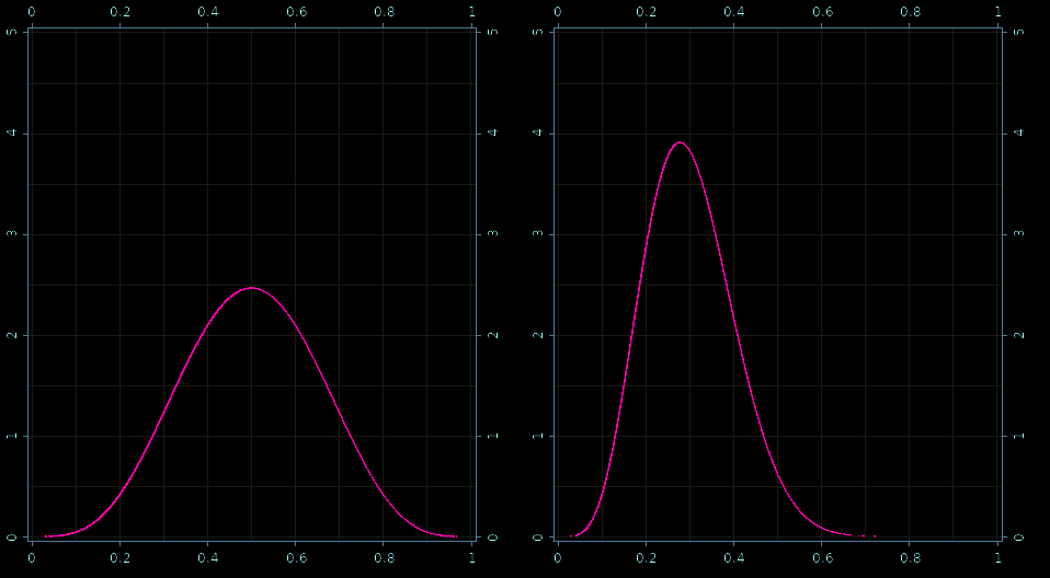
The coin example through simulation

• MCMC not necessary in this case
• Good as a hello world example
• Comparison with analytical solution

Run the analysis on the GPU

(def result (atom
(with-default-bayadera
  (let [a 5 b 5
        z 1 N 10]
    (with-release
      [prior-dist (beta a b)
       prior-sampler (sampler prior-dist)
       prior-sample (dataset (sample! prior-sampler))
       prior-pdf (pdf prior-dist prior-sample)
       post (posterior (posterior-model (:binomial likelihoods)
                                        (:beta distributions)))
       post-dist (post (sv (op (binomial-lik-params N z) (beta-params a b))))
       post-sampler (time (doto (sampler post-dist) (mix!)))
       post-sample (dataset (sample! post-sampler))
       post-pdf (scal! (/ 1.0 (evidence post-dist prior-sample))
                       (pdf post-dist post-sample))]

      {:prior {:sample (native (row (p/data prior-sample) 0))
               :pdf (native prior-pdf)}
       :posterior {:sample (native (row (p/data post-sample) 0))
                   :pdf (native post-pdf)}})))))

Prior and posterior - samples!

Real-World: Robust Linear Regression

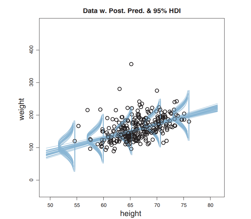
Hierarchical Model

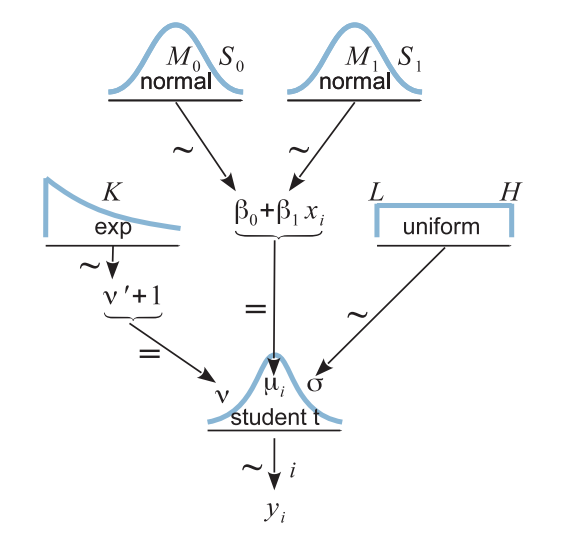
Resulting Posterior

Read the data

(defn read-data [in-file]
  (loop [c 0 data (drop 1 (csv/read-csv in-file)) hw (transient [])]
    (if data
      (let [[_ h w] (first data)]
        (recur (inc c) (next data)
               (-> hw (conj! (double (read-string h)))
                   (conj! (double (read-string w))))))
      (op [c] (persistent! hw)))))

(def params-300 (sv (read-data (slurp (io/file "ht-wt-data-300.csv")))))

#'user/read-data#'user/params-300

Create a custom model

(def rlr-source (slurp (io/file "robust-linear-regression.h")))

(def rlr-prior
  (cl-distribution-model [(:gaussian source-library)
                          (:uniform source-library)
                          (:exponential source-library)
                          (:t source-library)
                          rlr-source]
                         :name "rlr" :mcmc-logpdf "rlr_mcmc_logpdf"
                         :params-size 7 :dimension 4))

(defn rlr-likelihood [n]
  (cl-likelihood-model rlr-source :name "rlr" :params-size n))

#'user/rlr-source#'user/rlr-prior#'user/rlr-likelihood

Model's likelihood function

REAL rlr_loglik(__constant const REAL* params, REAL* x) {
    const REAL nu = x[0];
    const REAL b0 = x[1];
    const REAL b1 = x[2];
    const REAL sigma = x[3];
    const uint n = (uint)params[0];
    const bool valid = (0.0f < nu) && (0.0f < sigma);
    if (valid) {
        const REAL scale = t_log_scale(nu, sigma);
        REAL res = 0.0;
        for (uint i = 0; i < n; i = i+2) {
            res += t_log_unscaled(nu,
                                  b0 + b1 * params[i+1],
                                  sigma, params[i+2])
                + scale;
        }
        return res;
    }
    return NAN;
}

Model's prior function

REAL rlr_logpdf(__constant const REAL* params, REAL* x) {
    return exponential_log(params[0], x[0] - 1)
        + gaussian_log(params[1], params[2], x[1])
        + gaussian_log(params[3], params[4], x[2])
        + uniform_log(params[5], params[6], x[3]);

}

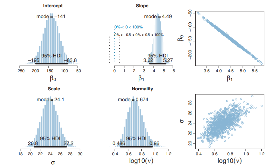
Running the inference on the GPU

(def result (atom
(with-default-bayadera
  (with-release
    [prior (distribution rlr-prior)
     prior-dist (prior (sv 10 -100 100 5 10 0.001 1000))

     post (posterior "rlr_300" (rlr-likelihood (dim params-300)) prior-dist)
     post-dist (post params-300)
     post-sampler (sampler post-dist {:limits (sge 2 4 [1 10 -400 100 0 20 0.01 100])})]

    (mix! post-sampler {:step 384})

    (histogram! post-sampler 1000)))))

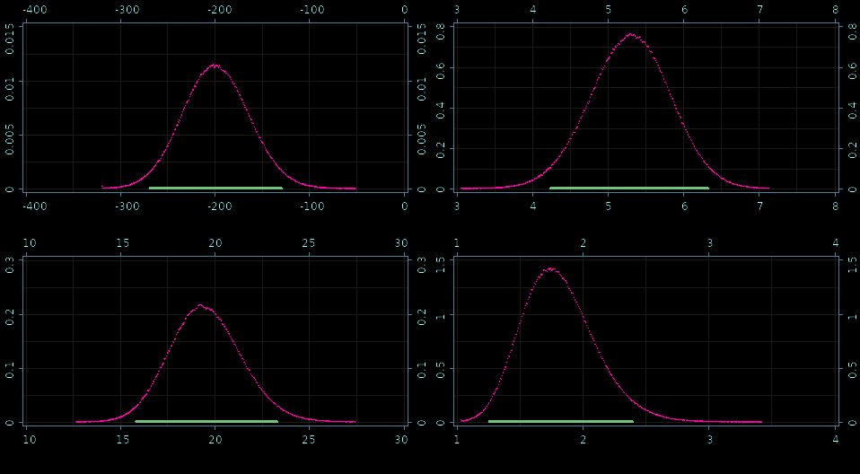
Generate posterior diagrams

(defn var-plot [] (plot2d (qa/current-applet) {:width 480 :height 240}))

(defn setup []
  (q/background 0)
  (q/image (show (render-histogram (var-plot) @result 1)) 0 0)
  (q/image (show (render-histogram (var-plot) @result 2)) 480 0)
  (q/image (show (render-histogram (var-plot) @result 3)) 0 260)
  (q/image (show (render-histogram (var-plot) @result 0)) 480 260)

  (q/save "robust-linear-regression.png"))

#_(q/defsketch diagrams :renderer :p2d :size :fullscreen
    :setup setup :middleware [pause-on-error])

Fine grained histograms!

Posteriors: β₀, β_1,σ, and ν

How fast is it?

• Bayadera
  • 61,208,576 samples in 267 ms.
  • 4.36 ns per (computationally heavy) sample
  • very precise histogram
• JAGS/Stan (state-of-the-art bayesian C++ tools)
  • 20,000 samples in 180/485 seconds
  • 9 ms per sample
  • rough histogram
• 2,000,000 × faster per sample
• more precise results, 1000 × faster

In real life

• 1 second vs a couple of hours
• 1 minute vs several days!
• 1 hour vs couple months/ a year

Thank You

The presentation can be reached through my blog:

• https://dragan.rocks

Find more at:

• https://bayadera.uncomplicate.org
• https://clojurecl.uncomplicate.org
• https://neanderthal.uncomplicate.org
• https://fluokitten.uncomplicate.org