Deep Learning from Scratch to GPU - 1 - Representing Layers and Connections

Below is a typical neural network diagram. As the story usually goes, we plug some input data in the Input Layer, and the network then propagates the signal through Hidden Layer 1 and Hidden Layer 2, using weighted connections, to produce the output at the Output Layer. For example, the input data is the pixels of an image, and the output are "probabilities" of this image belonging to a class, such as cat (\(y_1\)) or dog (\(y_2\)).

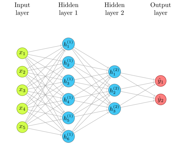
Neural Networks are often used to classify complex things such as objects in photographs, or to "predict" future data. Mechanically, though, there is no magic. They just approximate functions. What exactly are inputs and outputs is not particularly important at this moment. The network can approximate (or, to be fancy, "predict"), for example, even such mundane functions as \(y = sin(x_1) + cos(x_2)\).

Note that this is an instance of a transfer function. We provide an input, and the network propagates that signal to calculate the output; on the surface, just like any other function!

Different than everyday functions that we use, neural networks compute anything using only this architecture of nodes and weighted connections. The trick is in finding the right weights so that the approximation is close to the "right" value. This is what learning in deep learning is all about. For now, though, we are only dealing with inference, the process of computing the output using the given structure, input, and whatever weights there are.

The most straightforward thing to do, and the most naive error to make, is to read about analogies with neurons in the human brain, look at these diagrams, and try to model nodes and weighted connections as first-class objects. This might be a good approach with business oriented problems. First-class objects might bring the ultimate flexibility: each node and connection could have different polymorphic logic. That is the flexibility that we do not need. Even if that flexibility could help with better inference, it would be much slower, and training such a wandering network would be a challenge.

Rather than in such enterprising "neurons", the strength of neural networks is in their simple structure. Each node in a layer and each connection between two layers have exactly the same structure and logic. The only moving part are the numerical values in weights and thresholds. We can exploit that to create efficient implementations that fit well into hardware optimizations for numerical computations.

I'd say that the human brain analogy is more a product of marketing than a technical necessity. One layer of a basic neural network practically does logistic regression. There are more advanced structures, but the point is that they do not implement anything close to biological neurons.

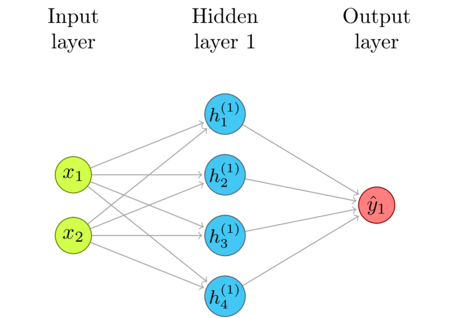
Let's just consider the input layer, the first hidden layer, and the connections between them.

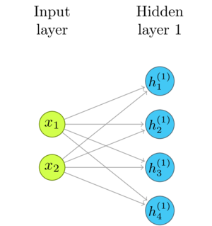
We can represent the input with a vector of two numbers, and the output of the Hidden Layer 1 with a vector of four numbers. Note that, since there is a weighted connection from each \(x_n\) to each \(h^{(1)}_m\), there are \(m\times{n}\) connections. The only data about each connection are its weight, and the nodes it connects. That fits well with what a matrix can represent. For example, the number at \(w_{21}\) is the weight between the first input, \(x_1\) and the second output, \(h^{(1)}_2\).

We compute the output of the first hidden layer in the following way:

Since you've read the Linear Algebra Refresher (1) - Vector Spaces that I recommended, you'll recognize that these are technically four dot products between the corresponding rows of the weight matrix and the input vector.

Conceptually, we can go further than low-level dot products: the weight matrix transforms the input vector into the hidden layer vector. I've written about matrix transformations in Linear Algebra Refresher (3) - Matrix Transformations.

We don't have to juggle indexes and program low-level loops. The basic matrix-vector product implements the propagation from each layer to the next!

For example, for some specific input and weights:

To try this in Clojure, we require some basic Neanderthal functions.

(require '[uncomplicate.commons.core :refer [with-release]]
         '[uncomplicate.neanderthal
           [native :refer [dv dge]]
           [core :refer [mv!]]])

The minimal code example, following the Yagni principle, would be something like this:

(with-release [x (dv 0.3 0.9)
               w1 (dge 4 2 [0.3 0.6
                            0.1 2.0
                            0.9 3.7
                            0.0 1.0]
                       {:layout :row})
               h1 (dv 4)]
  (println (mv! w1 x h1)))

#RealBlockVector[double, n:4, offset: 0, stride:1]
[   0.00    1.83    3.60    0.90 ]

The code does not need much explaining: w1, x, and h1 represent weights, input, and the first hidden layer. The function mv! applies the matrix transformation w1 to the vector x (by multiplying w1 by x; mv stands for "matrix times vector")

We should make sure that this code works well with large networks processed through lots of cycles when we get to implement the learning part, so we have to take care to reuse memory; thus we use the destructive version of mv, mv!. Also, the memory that holds the data is outside the JVM; thus we need to take care of its lifecycle and release it (automatically, using with-release) as soon it is not needed. This might not be important for such small examples, but is crucial in "real" use cases.

The output of the first layer is the input of the second layer:

(with-release [x (dv 0.3 0.9)
               w1 (dge 4 2 [0.3 0.6
                            0.1 2.0
                            0.9 3.7
                            0.0 1.0]
                       {:layout :row})
               h1 (dv 4)
               w2 (dge 1 4 [0.75 0.15 0.22 0.33])
               y (dv 1)]
  (println (mv! w2 (mv! w1 x h1) y)))

#RealBlockVector[double, n:1, offset: 0, stride:1]
[   1.84 ]

The final result is \(y_1=1.84\). What does it represent and mean? Which function does it approximate? Who knows. The weights I plugged in are not the result of any training nor insight. I've just pulled some random numbers out of my hat to show the computation steps.

The network we created is still a simple toy.

It's not even a proper multi-layer perceptron, since we did not implement non-linear activation of the outputs. Funnily enough, the nodes we have implemented are perceptrons, and there are multiple layers full of these. You'll soon get used to the tradition of inventing confusing and inconsistent grand-sounding names for every incremental feature in machine learning. Without non-linearity introduced by activations, we could stack thousands of layers, and our "deep" network would still perform only linear approximation equivalent to a single layer. If it is not clear to you why this happens, check out composition of transformations).

We have not implemented thresholds, or biases, yet. We've also left everything in independent matrices and vectors, without a structure involving layers that would hold them together. And we haven't even touched the learning part, which is 95% of the work. There are more things that are necessary, and even more things that are nice to have, and we'll cover these.

This code only runs on the CPU, but getting it to run on the GPU is rather easy. I'll show how to do this soon, but I bet you can even figure this on your own, with nothing more than Neanderthal Hello World example! There are posts on this blog showing how to do this, too.

My intention is to offer an easy start, so you do try this code. We will gradually apply and discuss each improvement in the following posts. Run this easy code on your own computer, and, why not, improve it in advance! The best way to learn is by experimenting and making mistakes.

I hope you're eager to continue to the next part: Bias and Activation Function

Clojurists Together financially supported writing this series. Big thanks to all Clojurians who contribute, and thank you for reading and discussing this series.