Deep Learning from Scratch to GPU - 2 - Bias and Activation Function

Need help with your custom Clojure software? I'm open to (selected) contract work.

February 11, 2019

Please share: Twitter.

These books fund my work! Please check them out.

If you haven't yet, read my introduction to this series in Deep Learning in Clojure from Scratch to GPU - Part 0 - Why Bother?.

The previous article, Part 1, is here: Representing Layers and Connections.

To run the code, you need a Clojure project with Neanderthal () included as a dependency. If you're in a hurry, you can clone Neanderthal Hello World project.

Don't forget to read at least some introduction from Neural Networks and Deep Learning, start up the REPL from your favorite Clojure development environment, and let's continue with the tutorial.

(require '[uncomplicate.commons.core :refer [with-release]]
         '[uncomplicate.fluokitten.core :refer [fmap!]]
         '[uncomplicate.neanderthal
           [native :refer [dv dge]]
           [core :refer [mv! mv axpy! scal!]]
           [math :refer [signum exp]]
           [vect-math :refer [fmax! tanh! linear-frac!]]])

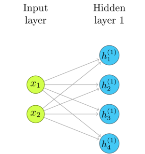
The Network Diagram

I'll repeat the basic diagram from the previous post, as a reference.

Threshold and Bias

In the current state, the network combines all layers into a single linear transformation. We can introduce basic decision-making capability by adding a cutoff to the output of each neuron. When the weighted sums of its inputs are below that threshold, the output is zero and when they are above, the output is one.

\begin{equation} output = \left\{ \begin{array}{ll} 0 & W\mathbf{x} \leq threshold \\ 1 & W\mathbf{x} > threshold \\ \end{array} \right. \end{equation}

Since we keep the current outputs in a (potentially) huge vector, it would be inconvenient to write a scalar-based logic for that. I prefer to use a vectorized function, or create one if there is not exactly what we need.

Neanderthal does not have the exact cutoff function, but we can create one by subtracting threshold from the maximum of each threshold and the signal value and then mapping the signum function to the result. There are simpler ways to compute this, but I wanted to use the existing functions, and do the computation in-place. It is of purely educational value, anyway. We will see soon that there are better things to use for transforming the output than the vanilla step function.

(defn step! [threshold x]
  (fmap! signum (axpy! -1.0 threshold (fmax! threshold x x))))

(let [threshold (dv [1 2 3])
      x (dv [0 2 7])]
  (step! threshold x))

nil#RealBlockVector[double, n:3, offset: 0, stride:1]
[   0.00    0.00    1.00 ]

I'm going to show you a few steps in the evolution of the code, so I will reuse weights and x. To simplify the example, we will use global def and not care about properly releasing the memory. It will not matter in a REPL session, but not forget to do it in the real code. Continuing the example from Part 1:

(def x (dv 0.3 0.9))
(def w1 (dge 4 2 [0.3 0.6
                  0.1 2.0
                  0.9 3.7
                  0.0 1.0]
             {:layout :row}))
(def threshold (dv 0.7 0.2 1.1 2))

Since we do not care about extra instances at the moment, we'll use the pure mv function instead of mv! for convenience. mv creates the resulting vector y, instead of mutating the one that has to be provided as an argument.

(step! threshold (mv w1 x))

nil#RealBlockVector[double, n:4, offset: 0, stride:1]
[   0.00    1.00    1.00    0.00 ]

The bias is simply the threshold moved to the left side of the equation:

\begin{equation} output = \left\{ \begin{array}{ll} 0 & W\mathbf{x} - bias \leq 0 \\ 1 & W\mathbf{x} - bias > 0 \\ \end{array} \right. \end{equation}

(def bias (dv 0.7 0.2 1.1 2))
(def zero (dv 4))

(step! zero (axpy! -1.0 bias (mv w1 x)))

nil#RealBlockVector[double, n:4, offset: 0, stride:1]
[   0.00    1.00    1.00    0.00 ]

Remember that bias is the same as threshold. There is no need for the extra zero vector.

(step! bias (mv w1 x))

nil#RealBlockVector[double, n:4, offset: 0, stride:1]
[   0.00    1.00    1.00    0.00 ]

Activation Function

The decision capabilities supported by the step function are rather crude. The neuron either outputs a constant value (1), or zero. It is better to use functions that offer different levels of the signal strength. Instead of the step function, the output of each neuron passes through an activation function. Countless functions can be an activation function, but a handful proved the best choice.

Like neural networks themselves, the functions that work well are simple. Activation functions have to be chosen carefully, to support the learning algorithms, most importantly to be easily differentiable. Until recently, the sigmoid and tanh functions were the top picks. Recently an even simpler function, ReLU, became the activation function of choice.

Rectified Linear Unit (\(ReLU\))

ReLU is short for Rectified Linear Unit. Sounds mysterious, but it is a straightforward linear function that has zero value below the threshold, which is typically zero.

\begin{equation} f(x) = max(0, x) \end{equation}

It's even simpler to implement than the step function, so we do this, if nothing else, for fun.

(defn relu! [threshold x]
  (axpy! -1.0 threshold (fmax! threshold x x)))

It might seem strange that I kept the threshold as an argument to the relu function. Isn't ReLU always cut-off at zero? Consider it a bit of optimization. There is no built-in optimize ReLU function. To implement the formula \(f(x) = max(0, x)\) we either have to use mapping over the max function, or to use the vectorized fmax, which requires an additional vector that holds the zeros. Since we need to subtract the biases anyway before the activation, by fusing these two phases, I avoided the need for maintaining the extra array of zeros. That may or may not be the best choice for the complete library, but since the main point of this blog is teaching, we stick to the Yagni principle.

(relu! bias (mv w1 x))

nil#RealBlockVector[double, n:4, offset: 0, stride:1]
[   0.00    1.63    2.50    0.00 ]

Hyperbolic Tangent (\(tanh\))

One popular activation function is tanh.

\begin{equation} tanh(x) = \frac{sinh(x)}{cosh(x)} = \frac{e^{2x} - 1}{e^{2x} + 1} \end{equation}

Note how it is close to the identity function \(f(x) = x\) in large part of the perimeter between \(-1\) and \(1\). As the absolute value of \(x\) gets larger, \(tanh(x)\) asymptotically approaches \(1\). Thus, the output is between \(-1\) and \(1\).

Since Neanderhtal has the vectorized variant of the tanh function in its vect-math, the implementation is easy.

(tanh! (axpy! -1.0 bias (mv w1 x)))

nil#RealBlockVector[double, n:4, offset: 0, stride:1]
[  -0.07    0.93    0.99   -0.80 ]

Sigmoid function

Until ReLU became popular, sigmoid was the most often used activation function. Sigmoid refers to a whole family of S-shaped functions, or, often, to a special case - the logistic function.

\begin{equation} S(x) = \frac{1}{1 + e^{-x}} = \frac{e^x}{e^{x} + 1} \end{equation}

Standard libraries often do not come with the implementation of the sigmoid function. We have to implement our own. We could implement it in the most straightforward way, just following the formula. That might be a good approach if we're only flexing our muscles, but may be not completely safe if we intend to use such implementation for the real work. (exp 710) is too big to fit even in double, while (exp 89) does not fit into float and produce an infinity (##Inf).

[(exp 709) (exp 710) (float (exp 88)) (float (exp 89))]

nil[8.218407461554972E307 ##Inf 1.6516363E38 ##Inf]

You can program that implementation as an exercise, and I'll show you another approach instead. Let me pull the following equality out of the magic mathematical hat, and ask you to believe me that it is true:

\begin{equation} S(x) = \frac{1}{2} + \frac{1}{2} \times tanh(\frac{x}{2}) \end{equation}

We can implement that easily by combining the vectorized tanh! and a bit of vectorized scaling.

(defn sigmoid! [x]
  (linear-frac! 0.5 (tanh! (scal! 0.5 x)) 0.5))

Let's program our layer with the logistic sigmoid activation.

(sigmoid! (axpy! -1.0 bias (mv w1 x)))

nil#RealBlockVector[double, n:4, offset: 0, stride:1]
[   0.48    0.84    0.92    0.25 ]

You can benchmark both implementations with large vectors, and see whether there is a difference in performance. I expect it to be only a fraction of the complete run time of the network. Consider that tanh(x) is safe, since it comes from a standard library, while you'll have to investigate whether the straightforward formula translation is good enough for what you want to do.

The next step

The layers of our fully connected network now go beyond linear transformations. We can stack as many as we'd like and do the inference.

(with-release [x (dv 0.3 0.9)
               w1 (dge 4 2 [0.3 0.6
                            0.1 2.0
                            0.9 3.7
                            0.0 1.0]
                       {:layout :row})
               bias1 (dv 0.7 0.2 1.1 2)
               h1 (dv 4)
               w2 (dge 1 4 [0.75 0.15 0.22 0.33])
               bias2 (dv 0.3)
               y (dv 1)]
  (tanh! (axpy! -1.0 bias1 (mv! w1 x h1)))
  (println (sigmoid! (axpy! -1.0 bias2 (mv! w2 h1 y)))))

#RealBlockVector[double, n:1, offset: 0, stride:1]
[   0.44 ]

This is getting repetitive. For each layer we add, we have to herd a few more disconnected matrices, vectors, and activation functions in place. In the next article, we will fix this by abstracting it into easy to use layers.

After that, we will make a few minor adjustments that enable our code to run on the GPU, just to make sure that it is easy to do.

Then we will be ready to tackle the 95% of the work: create the code for learning these weights from data, so that the numbers that the network compute become relevant.

The next article: Fully Connected Inference Layers.

Thank you

Clojurists Together financially supported writing this series. Big thanks to all Clojurians who contribute, and thank you for reading and discussing this series.