Deep Learning from Scratch to GPU - 3 - Fully Connected Inference Layers

We'll update the neural network diagram, to reflect the recently included biases and activation functions.

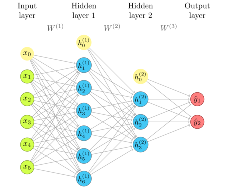
In each layer, bias is shown as an additional, "zero"-indexed, node, which, connected to nodes in the next layer, gives the bias vector. I haven't explicitly shown activation functions to avoid clutter. Consider that each node has activation at the output. If a layer didn't have any activation whatsoever, it would have been redundant (see composition of transformations).

We need a structure that keeps the account of the weights, biases and output of each layer. It should manage the life-cycle and release that memory space when appropriate. That structure can implement Clojure's IFn interface, so we can invoke it as any regular Clojure function.

(import 'clojure.lang.IFn)

We will create FullyConnectedInference as a Clojure type, which gets compiled into a Java class. FullyConnectedInference implements the release method of the Releaseable protocol, and the invoke method of IFn. We would also like to access and see the weights and bias values so we create new protocol, Parameters, with weight and bias methods.

(defprotocol Parameters
  (weights [this])
  (bias [this]))

(deftype FullyConnectedInference [w b h activ-fn]
  Releaseable
  (release [_]
    (release w)
    (release b)
    (release h))
  Parameters
  (weights [this] w)
  (bias [this] b)
  IFn
  (invoke [_ x]
    (activ-fn b (mv! w x h))))

At the time of creation, each FullyConnectedInference need to be supplied with an activation function, the matrix for weights, and vectors for bias and output that have matching dimensions. Of course, we will automate that process.

(defn fully-connected [activ-fn in-dim out-dim]
  (let-release [w (dge out-dim in-dim)
                bias (dv out-dim)
                h (dv out-dim)]
    (->FullyConnectedInference w bias h activ-fn)))

Now a simple call to the fully-connected function that specifies the activation function and the dimensions of input dimension (number of neurons in the previous layer) and output dimension (the number of neurons in this layer) will create and properly initialize it.

let-release is a variant of let that releases its bindings (w, bias, and/or h) if anything goes wrong and an exception gets thrown in its scope. with-release, on the other hand, releases the bindings in all cases.

We can use a few matching functions that we discussed in the previous article.

(defn activ-sigmoid! [bias x]
  (axpy! -1.0 bias x)
  (linear-frac! 0.5 (tanh! (scal! 0.5 x)) 0.5))

(defn activ-tanh! [bias x]
  (tanh! (axpy! -1.0 bias x))  )

Now we are ready to re-create the existing example in a more convenient form. Note that we no longer have to worry about creating the matching structures of a layer; it happens automatically when we create each layer. I use the transfer! function to set up the values of weights and bias, but typically these values will already be there after the training (learning) of the network. Here we are using the same "random" numbers as before as a temporary testing crutch.

(with-release [x (dv 0.3 0.9)
               layer-1 (fully-connected activ-sigmoid! 2 4)]
  (transfer! [0.3 0.1 0.0 0.0 0.6 2.0 3.7 1.0] (weights layer-1))
  (transfer! (dv 0.7 0.2 1.1 2) (bias layer-1))
  (println (layer-1 x)))

#RealBlockVector[double, n:4, offset: 0, stride:1]
[   0.48    0.84    0.90    0.25 ]

The output is the same as before, as we expected.

Note that the layer is a transfer function that, given the input, computes and returns the output. Like with other Clojure functions, the output value can be an input to the next layer function.

(with-release [x (dv 0.3 0.9)
               layer-1 (fully-connected activ-tanh! 2 4)
               layer-2 (fully-connected activ-sigmoid! 4 1)]
  (transfer! [0.3 0.1 0.9 0.0 0.6 2.0 3.7 1.0] (weights layer-1))
  (transfer! [0.7 0.2 1.1 2] (bias layer-1))
  (transfer! [0.75 0.15 0.22 0.33] (weights layer-2))
  (transfer! [0.3] (bias layer-2))
  (println (layer-2 (layer-1 x))))

#RealBlockVector[double, n:1, offset: 0, stride:1]
[   0.44 ]

If we don't count the transfer! calls, we have 3 lines of code that describe the whole network: two lines to create the layers, and one line for the nested call of layers as functions. It is already concise, and we will still improve it in the upcoming articles.

With rather small networks consisting of a few layers with few neurons each, any implementation will be fast. Let's create a network with a larger number of neurons, to get a feel of how fast we can expect these things to run.

Here is a network with input dimension of 10000. The exact numbers are not important, since the example is superficial, but you can imagine that 10000 represents an image that has 400 × 250 pixels. I've put 5000 neurons in the first layer, 1000 in the second layer, and 10 at the output. Just some random large-ish dimensions. Imagine 10 categories at the output.

(with-release [x (dv 10000)
               layer-1 (fully-connected activ-tanh! 10000 5000)
               layer-2 (fully-connected activ-sigmoid! 5000 1000)
               layer-3 (fully-connected activ-sigmoid! 1000 10)]
  ;; Call it like this:
  ;; (quick-bench (layer-3 (layer-2 (layer-1 x))))
  (layer-3 (layer-2 (layer-1 x))))

Evaluation count : 36 in 6 samples of 6 calls.
             Execution time mean : 18.320566 ms
    Execution time std-deviation : 1.108914 ms
   Execution time lower quantile : 17.117256 ms ( 2.5%)
   Execution time upper quantile : 19.847416 ms (97.5%)
                   Overhead used : 7.384194 ns

On my 5 year old CPU (i7-4790k), one inference through this network takes 18 milliseconds. If you have another neural networks library at hand, you could construct the same network (virtually any NN software should support this basic structure) and compare the timings.

So far so good. 18 ms should not be slow. But what if we have lots of data to process? Does that mean that if I have 10 thousand inputs, I'd need to make a loop that invokes this inference 10 thousand times with different input, and wait 3 minutes for the results?

Is the way to speed that up putting it on the GPU? We'll do that later, but there is something that we can do even on the CPU to improve this! That's the topic of the next article, Increasing Performance with Batch Processing!

Clojurists Together financially supported writing this series. Big thanks to all Clojurians who contribute, and thank you for reading and discussing this series.