Deep Learning from Scratch to GPU - 13 - Initializing Weights
April 10, 2019
Please share this post in your communities. Without your help, it will stay burried under tons of corporate-pushed, AI and blog farm generated slop, and very few people will know that this exists.
These books fund my work! Please check them out.


As the iterative learning algorithm has to start somewhere, we have to decide how to initialize weights. Here we try a few techniques and weight their strengths and weaknesses until we find one that is good enough.
If you haven't yet, read my introduction to this series in Deep Learning in Clojure from Scratch to GPU - Part 0 - Why Bother?.
The previous article, Part 12, is here: A Simple Neural Network Training API.
To run the code, you need a Clojure project with Neanderthal () included as a dependency. If you're in a hurry, you can clone Neanderthal Hello World project.
Don't forget to read at least some introduction from Neural Networks and Deep Learning, start up the REPL from your favorite Clojure development environment, and let's continue with the tutorial.
Why properly initialized weights are important
So far, we have seen how a neural network is a series of linear transformations interposed with non-linear activations.
Here's simple example, an one layer network we used in part 1, Representing Layers and Connections:
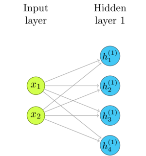
Take a look at the formula for the linear transformations that we defined in that article:
\(\mathbf{h} = W\mathbf{x}\)
Each \(h_i\) is a dot product of the respective row of \(W\) and the input.
\begin{gather*} h^{(1)}_1 = w_{11}\times{} x_1 + w_{12}\times{} x_2\\ h^{(1)}_2 = w_{21}\times{} x_1 + w_{22}\times{} x_2\\ h^{(1)}_3 = w_{31}\times{} x_1 + w_{32}\times{} x_2\\ h^{(1)}_4 = w_{41}\times{} x_1 + w_{42}\times{} x_2\\ \end{gather*}Until now, we have set the initial weights and inputs to be in the range \([0, 1]\), as in the following example that you have seen many times by now.
(with-release [x (ge native-float 2 2 [0.3 0.9 0.3 0.9])
               y (ge native-float 1 2 [0.50 0.50])
               inference (inference-network
                          native-float 2
                          [(fully-connected 4 tanh)
                           (fully-connected 1 sigmoid)])
               inf-layers (layers inference)
               training (training-network inference x)]
  (transfer! [0.3 0.1 0.9 0.0 0.6 2.0 3.7 1.0] (weights (inf-layers 0)))
  (transfer! [0.7 0.2 1.1 2] (bias (inf-layers 0)))
  (transfer! [0.75 0.15 0.22 0.33] (weights (inf-layers 1)))
  (transfer! [0.3] (bias (inf-layers 1)))
  (sgd training y quadratic-cost! 2000 0.05)
  (transfer (inference x)))
nil#RealGEMatrix[float, mxn:1x2, layout:column, offset:0]
   ▥       ↓       ↓       ┓
   →       0.50    0.50
   ┗                       ┛
As all operands are between 0 and 1, the dot products \(h\) are likely to be in that range, or at least not much larger.
If any of the weights \(w\) or inputs \(x\) are large numbers, \(h\) also has a chance to be large. If the network didn't have non-linear activations, the inputs to the following layer would grow uncontrollably, which would propagate further. Some activation functions, such as ReLU, are linear in the positive domain, so this would propagate to the output. The sigmoid and hyperbolic tangent activation functions would saturate at \(1\) at the upper bound and \(0\) or \(-1\) at the lower bound.
Although the saturation will contain the inputs to the next layer to the \([-1,1]\) range, it would make the learning difficult, since the saturated functions would have problems propagating the gradients backwards.
We are still using a trivial example, which can easily illustrate this problem (that's why I'm still keeping it, despite it being silly). Just change the weights to be numbers larger than one. Even though we are just chasing one input/output example (\((0.3, 0.9) \mapsto 0.5\)) where there is nothing even remotely challenging to learn, our algorithm gets stuck in the saturation zone right away.
(with-release [x (ge native-float 2 2 [0.3 0.9 0.3 0.9])
               y (ge native-float 1 2 [0.50 0.50])
               inference (inference-network
                          native-float 2
                          [(fully-connected 4 tanh)
                           (fully-connected 1 sigmoid)])
               inf-layers (layers inference)
               training (training-network inference x)]
  (transfer! [3 1 9 0 6 20 37 10] (weights (inf-layers 0)))
  (transfer! [7 2 11 2] (bias (inf-layers 0)))
  (transfer! [75 15 22 33] (weights (inf-layers 1)))
  (transfer! [3] (bias (inf-layers 1)))
  (sgd training y quadratic-cost! 2000 0.05)
  (transfer (inference x)))
nil#RealGEMatrix[float, mxn:1x2, layout:column, offset:0]
   ▥       ↓       ↓       ┓
   →       0.00    0.00
   ┗                       ┛
It is obvious that we should keep the average absolute value of weights below 1. But, how small should they be? If weights are too small, the signal will be feeble. Feeble signal might not have problems in small networks, but when passed through a large number of layers, it would be dampened before reaching the output. I'd need a larger example to illustrate it, so for this one I'd have to ask you to trust me.
Let's say that 0.001 is not too small, and yet not too large. Why don't we pick a universally good value and set all weights to it? The problem with that approach is that all neurons would behave in the same manner. We wouldn't have a variability in the neurons that is needed for proper learning.
Although there is not a universal best strategy for setting weighs, a few things are certain enough:
- 1) it should be done automatically
- 2) the values should be small enough to avoid saturation
- 3) the values should be large enough to be able to propagate the signal
- 4) the initial weights should be random
Generating random numbers
As we are going to need a lot of random numbers, it is a good time to see about generating
them. Clojure, as most programming languages, have a function that returns uniformly distributed
random numbers - rand. It is important to note that these are pseudo random numbers! They are generated by deterministic
algorithms, and only appear to be random. The default algorithms used in standard libraries are good enough
for most casual uses but are not of high quality. They are certainly not good enough for cryptography, but,
luckily, we are not trying to outsmart NSA. They are not even good enough for serious simulations.
For this illustration, rand is OK.
The default rand signature returns uniformly distributed numbers between 0 and 1. It is
easy enough to produce a sequence of random numbers.
(map rand (repeat 10 1))
nil(0.7014240191763038 0.6202193837181832 0.1714819863895033 0.6762836795545388 0.11935216796634984 0.6572938157260321 0.16449131618304536 0.5318560880392705 0.7310647135005525 0.45385262971843154)
(require '[uncomplicate.fluokitten.core :refer [fmap!]])
Since Fluokitten's fmap! function supports matrices, we can populate an existing matrix
with random numbers by simply fmap! ing rand over it, while ignoring the old entry values of the matrix.
(fmap! (fn [_] (rand)) (fge 3 2))
nil#RealGEMatrix[float, mxn:3x2, layout:column, offset:0]
   ▥       ↓       ↓       ┓
   →       0.83    0.48
   →       0.12    0.79
   →       0.45    0.85
   ┗                       ┛
The previous implementation used number boxing. Neanderthal supports primitive arguments,
and by annotating the function arguments with double, we can avoid boxing and make this
faster by almost an order of magnitude.
(defn rand-uniform ^double [^double _]
  (double (rand)))
Let's try to initialize all weights with uniform random numbers between \(0\) and \(1\).
(with-release [x (ge native-float 2 2 [0.3 0.9 0.3 0.9])
               y (ge native-float 1 2 [0.50 0.50])
               inference (inference-network
                          native-float 2
                          [(fully-connected 4 tanh)
                           (fully-connected 1 sigmoid)])
               inf-layers (layers inference)
               training (training-network inference x)]
  (fmap! rand-uniform (weights (inf-layers 0)))
  (fmap! rand-uniform (bias (inf-layers 0)))
  (fmap! rand-uniform (weights (inf-layers 1)))
  (fmap! rand-uniform (bias (inf-layers 1)))
  (sgd training y quadratic-cost! 2000 0.05)
  (transfer (inference x)))
nil#RealGEMatrix[float, mxn:1x2, layout:column, offset:0]
   ▥       ↓       ↓       ┓
   →       0.02    0.02
   ┗                       ┛
It does not help much. This network still saturates most of the times when I call it. The reason is that, for example, \(0.9*0.4 + 0.8*0.75 + 0.1*0.3 + 0.6*0.9\) is still \(1.53\) which saturates the sigmoid or tanh activation.
We should avoid having too many large weights1. Most weighs should be small, only occasionally close to 1, and sometimes, rarely, even larger than 1. Yes, weights larger than 1 are useful. They can signify the importance of a particularly influential input.
Generating normally distributed random numbers
The answer is in the Gaussian distribution, also known as Normal distribution. I am sure that you've heard of the bell-shaped curve.
\begin{equation} X \sim \mathcal{N}(\mu,\,\sigma^{2})\,.\\ P(x) = \frac{1}{\sqrt{ 2\pi \sigma^2 }} e^{- \frac{(x - \mu)^2}{2\sigma ^2}} \end{equation}
When this curve represents the distribution, \(y\) axis shows the probability of a value \(x\). I deliberately avoided labeling the axes, because the point is that the width, height, and the position of this curve can be varied with the parameters mean (\(\mu\)) and standard deviation (\(\sigma\)). Mean determines the center of this curve, where the probability is highest. We want this to be 0. The standard deviation describes the "width" of this distribution. The smaller it is, more values will be closer to mean.
The Gaussian distribution with mean \(0\) and standard deviation \(1\) is called Standard normal distribution.
\begin{equation} X \sim \mathcal{N}(0,1)\,.\\ P(x) = \frac{1}{\sqrt{2\pi}} e^{- \frac{1}{2}x^2} \end{equation}If we could generate a sample from the standard normal distribution, we could easily scale the width. The first task is, then, to find a way to generate such numbers.
The bad news is that the generator for the normal distribution is not a part of the standard library. The good news is that there are simple algorithms to produce normally distributed samples from uniformly distributed samples. This is a strike of good luck, since we can do that only for a few distributions. For most distributions, we have to do simulations such as MCMC (check out Bayadera if you need this!).
One of the methods to generate random Gaussian numbers from uniformly distributed numbers that we already know how to generate is the Box-Muller transform. If I have two uniformly distributed numbers, \(U1\) and \(U2\), I can produce two normally distributed numbers, \(Z1\) and \(Z2\) using these formulas:
\begin{equation} Z_1 = \sqrt{-2 \ln U1} \cos(2\pi U_2)\\ Z_2 = \sqrt{-2 \ln U1} \sin(2\pi U_2) \end{equation}
Fine, sin, cos, and log are the functions that we have in Neanderthal, in both
scalar and vectorized form.
(require '[uncomplicate.neanderthal
           [vect-math :refer [tanh! linear-frac! sqr! mul!]]
           [math :refer [sqrt log sin pi sqr]]])
The following function generates two uniformly distributed random numbers, and uses them to produce one from the normal distribution. It wastes one number, but I wanted to keep the implementation simple and compatible with the previous setup for generating uniformly distributed numbers.
(defn rand-gaussian ^double [^double _]
  (let [u1 (rand-uniform Double/NaN)
        u2 (rand-uniform Double/NaN)]
    (double (* (sqrt (* -2.0 (log u1))) (sin (* 2.0 pi u2))))))
The same example works better now.
(with-release [x (ge native-float 2 2 [0.3 0.9 0.3 0.9])
               y (ge native-float 1 2 [0.50 0.50])
               inference (inference-network
                          native-float 2
                          [(fully-connected 4 tanh)
                           (fully-connected 1 sigmoid)])
               inf-layers (layers inference)
               training (training-network inference x)]
  (fmap! rand-gaussian (weights (inf-layers 0)))
  (fmap! rand-gaussian (bias (inf-layers 0)))
  (fmap! rand-gaussian (weights (inf-layers 1)))
  (fmap! rand-gaussian (bias (inf-layers 1)))
  (sgd training y quadratic-cost! 2000 0.05)
  (transfer (inference x)))
nil#RealGEMatrix[float, mxn:1x2, layout:column, offset:0]
   ▥       ↓       ↓       ┓
   →       0.01    0.01
   ┗                       ┛
Although this initialization may work well with this trivial example, it fails often enough. The weights initialized with standard deviation \(\sigma = 1\) are still too large. We have to scale them down with respect to the number of neurons in the layer.
Automatically initializing weights
Now that we know how to generate random numbers from the appropriate distribution, it's time to automate this functionality.
(require '[uncomplicate.commons
           [core :refer [with-release let-release Releaseable release]]
           [utils :refer [direct-buffer]]]
         '[uncomplicate.clojurecuda.core :as cuda
           :refer [current-context default-stream synchronize!]]
         '[uncomplicate.clojurecl.core :as opencl
           :refer [*context* *command-queue* finish!]]
         '[uncomplicate.neanderthal.internal.api :refer [native-factory device]]
         '[uncomplicate.neanderthal
           [core :refer [mrows ncols dim raw view view-ge vctr copy row
                         entry! axpy! copy! scal! mv! transfer! transfer
                         mm! rk! view-ge vctr ge trans nrm2]]
           [math :refer [sqrt log sin pi sqr sqrt]]
           [vect-math :refer [tanh! linear-frac! sqr! mul! cosh! inv!]]
           [native :refer [fge native-float native-double]]
           [block :refer [buffer]]
           [cuda :refer [cuda-float]]
           [opencl :refer [opencl-float]]]
         '[criterium.core :refer [quick-bench]])
(import 'clojure.lang.IFn
        'uncomplicate.neanderthal.internal.host.MKL)
(defn init-layer! [layer!]
  (let [w (weights layer!)]
    (scal! (sqrt (/ 2.0 (+ (mrows w) (ncols w)))) (fmap! rand-gaussian w))
    (fmap! rand-gaussian (bias layer!))
    layer!))

(defn init! [network!]
  (doseq [layer (layers network!)]
    (init-layer! layer))
  network!)
Xavier Initialization
The function init-layer! extracts weights and biases from the layer and simply delegates
the job to the appropriate fmap! and rand-gaussian. We are using the Gaussian distribution with mean 0.
The standard deviation has to be scaled down, proportionally to the number of neurons in the layer,
to keep the expected value of the output in the safe zone.
The scaling of the standard deviation is not as straightforward as it seems. There are two trade-offs to consider: the signal that propagates forward favors scaling by the number of inputs. However, to preserve the gradients flowing backwards, we should scale proportionally to the number of outputs.
A widely accepted solution, the Xavier initialization, suggests drawing numbers from the distribution with the variance \(Var[W^L] = \frac{2}{n_{in}+n_{out}}\). It can be applied with both uniform and normal distribution.
We will use normal distribution, so this boils down to dividing the sample generated with \(\sigma = 1\) by the square root of 2 divided by the sum of inputs and outputs to the layer.
In theory, this initialization should be the best we implemented so far. Let's try it.
(with-release [x (ge native-float 2 2 [0.3 0.9 0.3 0.9])
               y (ge native-float 1 2 [0.50 0.50])
               inference (init! (inference-network
                                 native-float 2
                                 [(fully-connected 4 tanh)
                                  (fully-connected 1 sigmoid)]))
               training (training-network inference x)]
  (sgd training y quadratic-cost! 2000 0.05)
  (transfer (inference x)))
nil#RealGEMatrix[float, mxn:1x2, layout:column, offset:0]
   ▥       ↓       ↓       ┓
   →       0.50    0.50
   ┗                       ┛
This may work well, but it may also fail. Is our implementation wrong? I hope it is not. Please note that this is a network consisting of tiny layers. Therefore, the generated weights could often be close to one, and when scaled, they are scaled only by 0.57 and 0.63.
This makes this artificial example obsolete for our purposes. It served us well, but in the next article, with the infrastructure that we now have we can create something a bit more realistic. Then, we will see whether our implementation proves capable, and get hints for further improvements.
How fast is random number generation
Before we continue, we should check the efficiency of our weights initialization algorithm.
Uniformly distributed random numbers
I'll generate a matrix of 10,000 elements. It is large enough to represent something that we might see in the wild.
(with-release [x (ge native-double 100 100)]
  ;; (quick-bench (fmap! rand-uniform x)) ;; call quick bench
  (fmap! rand-uniform x))
Execution time mean : 1.250046 ms
I've varied dimensions a bit, and it seems to take around 125 ns per entry.
Normally distributed random numbers
Recall that, when we generate Gaussian random numbers, we throw away half of the uniform samples, and call some square roots, logarithms, sinuses and/or cosinuses.
(with-release [x (ge native-double 100 100)]
  ;; (quick-bench (fmap! rand-gaussian x)) ;; call quick bench
  (fmap! rand-gaussian x))
Execution time mean : 2.620225 ms
This is twice as slow. Knowing how we generate these numbers, this is even good.
Random number generation on the GPU
Our implementation can not be run on the GPU, unfortunately. The source of uniform random numbers, Clojure's
rand function, is available only on the CPU.
It turns out that random number generation on the GPU is rather tricky. The strength of GPU processing is in parallelization. Unfortunately, almost all pseudo-random generators rely on the state of the generator to produce the next random number. If dozens, thousands, or millions of processors are to generate random numbers, that would mean that their access to the state must be coordinated. This is a disaster to parallelism.
Fortunately, there are algorithms that avoid such problems. Unfortunately, the implementation is too complex to show here. I implemented some good ones, and this is available in Bayadera. I will include this into a deep learning library that I'm going to release (Yes, that might be a good news! If you are rooting for it to see the light of day sooner rather than later, and would like to support my work on it, please donate on my Patreon page.
For this tutorial, though, we would have to resort to generating the random numbers in the main memory using CPU and transferring them to the GPU memory.
(defn init-weights! [w b]
  (scal! (/ 1.0 (ncols w)) (fmap! rand-gaussian w))
  (fmap! rand-gaussian b))

(defn init-layer! [layer!]
  (let [w (weights layer!)
        b (bias layer!)]
    (if (= :cpu (device w))
      (init-weights! w b)
      (with-release [native-w (ge (native-factory w) (mrows w) (ncols w))
                     native-b (vctr (native-factory b) (dim b))]
        (init-weights! native-w native-b)
        (transfer! native-w w)
        (transfer! native-b b)))
    layer!))

(defn init! [network!]
  (doseq [layer (layers network!)]
    (init-layer! layer))
  network!)
Although this implementation is not ideal, it works on all devices.
(cuda/with-default
  (with-release [factory (cuda-float (current-context) default-stream)]
    (with-release [x (ge factory 10000 10000)
                   y (entry! (ge factory 10 10000) 0.33)
                   inference (time (init! (inference-network
                                           factory 10000
                                           [(fully-connected 5000 tanh)
                                            (fully-connected 1000 sigmoid)
                                            (fully-connected 10 sigmoid)])))
                   training (training-network inference x)]
      (time
         (sgd training y quadratic-cost! 10 0.05)))))
"Elapsed time: 14344.241479 msecs"
"Elapsed time: 2303.362116 msecs"
It took a lot of time to initialize these weights. The weights are initialized
in the main memory (using the slow-ish JVM math sin and ln functions, wasting the half of the uniform sample)
and then transferred to GPU memory. It is not a major problem right now,
since we're doing it only once, regardless of how many training epochs we run.
Also, the network is gigantic. In more realistic cases, the layer sizes would
be much smaller and this time less noticeable.
Bayadera would do this in a matter of milliseconds. But, there is a way to speed this thing up even if we use CPU for the random number generation.
In the following code, I use an internal function from Neanderthal. It is still not available in the public API, so don't rely on it, but I'm showcasing it anyway. For proper RNG, Bayadera is the right choice.
(let-release [stream (direct-buffer Long/BYTES)
              params (vctr native-float [0 1])]
  (let [seed (rand-int 1000)
        err (MKL/vslNewStreamARS5 seed stream)]
    (if (= 0 err)
      (defn float-gaussian-sample! [res]
        (let [err (MKL/vsRngGaussian stream (dim res) (buffer res) (buffer params))]
          (if (= 0 err)
            res
            (throw (ex-info "MKL error." {:error-code err})))))
      (ex-info "MKL error." {:error-code err}))))

(defn init-weights! [w b]
  (scal! (/ 1.0 (ncols w)) (float-gaussian-sample! w))
  (float-gaussian-sample! b))

(defn init-layer! [layer!]
  (let [w (weights layer!)
        b (bias layer!)]
    (if (= :cpu (device w))
      (init-weights! w b)
      (with-release [host-w (ge (native-factory w) (mrows w) (ncols w))
                     host-b (vctr (native-factory b) (dim b))]
        (init-weights! host-w host-b)
        (transfer! host-w w)
        (transfer! host-b b)))
    layer!))

(defn init! [network!]
  (doseq [layer (layers network!)]
    (init-layer! layer))
  network!)
I'm repeating the last example, which executes the learning algorithm on the GPU. Weights are still being generated on the CPU, but now by a fast internal implementation. What once took 80% of the running time, now takes 10%, which makes it good enough.
(cuda/with-default
  (with-release [factory (cuda-float (current-context) default-stream)]
    (with-release [x (ge factory 10000 10000)
                   y (entry! (ge factory 10 10000) 0.33)
                   inference (time (init! (inference-network
                                           factory 10000
                                           [(fully-connected 5000 tanh)
                                            (fully-connected 1000 sigmoid)
                                            (fully-connected 10 sigmoid)])))
                   training (training-network inference x)]
      (time
         (sgd training y quadratic-cost! 10 0.05)))))
"Elapsed time: 209.036422 msecs"
"Elapsed time: 2310.606784 msecs"
This might even be acceptable! I apologize (again!) for using some internal Neanderthal functions (that you're not supposed to) for this demonstration, but with these, we improved the weight initialization performance several dozen times compared to JVM-based one, even without a GPU RNG.
Check the final implementation
I'll check the final implementation again, just to make sure that we haven'd made some grave mistake in adapting the code to be able to serve both CPU and GPU based networks.
(with-release [x (ge native-float 2 2 [0.3 0.9 0.3 0.9])
               y (ge native-float 1 2 [0.50 0.50])
               inference (init! (inference-network
                                 native-float 2
                                 [(fully-connected 4 tanh)
                                  (fully-connected 1 sigmoid)]))
               training (training-network inference x)]
  (sgd training y quadratic-cost! 2000 0.05)
  (transfer (inference x)))
nil#RealGEMatrix[float, mxn:1x2, layout:column, offset:0]
   ▥       ↓       ↓       ┓
   →       0.50    0.50
   ┗                       ┛
It seems it works, although the example is so trivial, it easily saturates.
Donations
If you feel that you can afford to help, and wish to donate, I even created a special Starbucks for two tier at patreon.com/draganrocks. You can do something even cooler: adopt a pet function.
The next article
We finally have a somewhat complete API and its implementation. There are optimizations to add, but even without that, it should be useful for experimenting. With a handful of lines of code, we can create the network, and train in on some data. Is it going to learn well? I guess it will, at least when the task is simple.
Well, then, let's try it and learn a regression on some simple function in the next article!
Thank you
Clojurists Together financially supported writing this series. Big thanks to all Clojurians who contribute, and thank you for reading and discussing this series.