Deep Learning from Scratch to GPU - 12 - A Simple Neural Network Training API
April 3, 2019
Please share this post in your communities. Without your help, it will stay burried under tons of corporate-pushed, AI and blog farm generated slop, and very few people will know that this exists.
These books fund my work! Please check them out.


The stage has been set for wrapping up the simplest version of a complete neural network API, and its key part that offers the entry for the learning functionality: the training API.
If you haven't yet, read my introduction to this series in Deep Learning in Clojure from Scratch to GPU - Part 0 - Why Bother?.
The previous article, Part 11, is here: A Simple Neural Network API.
To run the code, you need a Clojure project with Neanderthal () included as a dependency. If you're in a hurry, you can clone Neanderthal Hello World project.
Don't forget to read at least some introduction from Neural Networks and Deep Learning, start up the REPL from your favorite Clojure development environment, and let's continue with the tutorial.
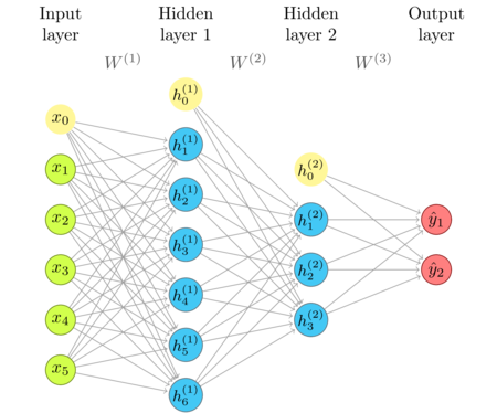
The network diagram
I'm repeating the network diagram from the previous article as a convenient reference.
Defining a simple NN API
Here's a draft of how using a NN API could look like, based on what we implemented a few days ago, in part 11, A Simple Neural Network API.
...
(def input (fv 1000))
(def output (fv 8))
(def inference (inference-network
                factory 1000
                [(fully-connected 256 sigmoid)
                 (fully-connected 64 tanh)
                 (fully-connected 16 sigmoid)]))
(def train (training inference input))
(sgd train output quadratic-cost 20 0.05)
...
The existing pieces
The imports and requires that we will need today are here.
(require '[uncomplicate.commons.core
           :refer [with-release let-release Releaseable release]]
         '[uncomplicate.clojurecuda.core :as cuda
           :refer [current-context default-stream synchronize!]]
         '[uncomplicate.clojurecl.core :as opencl
           :refer [*context* *command-queue* finish!]]
         '[uncomplicate.neanderthal
           [core :refer [mrows ncols dim raw view view-ge vctr copy row
                         entry! axpy! copy! scal! mv! transfer! transfer
                         mm! rk! view-ge vctr ge trans nrm2]]
           [math :refer [sqr]]
           [vect-math :refer [tanh! linear-frac! sqr! mul! cosh! inv!]]
           [native :refer [fge native-float]]
           [cuda :refer [cuda-float]]
           [opencl :refer [opencl-float]]])
(import 'clojure.lang.IFn)
I include the complete implementation we have by now, since this article is auto-generated from live code.
(defprotocol Parameters
  (weights [this])
  (bias [this]))

(defprotocol ActivationProvider
  (activation-fn [this]))

(deftype FullyConnectedInference [w b activ-fn]
  Releaseable
  (release [_]
    (release w)
    (release b)
    (release activ-fn))
  Parameters
  (weights [_] w)
  (bias [_] b)
  ActivationProvider
  (activation-fn [_] (activ-fn))
  IFn
  (invoke [_ x ones a]
    (activ-fn (rk! -1.0 b ones (mm! 1.0 w x 0.0 a)))))

(defn fully-connected [factory activ-fn in-dim out-dim]
  (let-release [w (ge factory out-dim in-dim)
                bias (vctr factory out-dim)]
    (->FullyConnectedInference w bias activ-fn)))

(defprotocol Backprop
  (forward [this])
  (backward [this eta]))

(defprotocol Transfer
  (input [this])
  (output [this])
  (ones [this]))

(defprotocol Activation
  (activ [_ z a!])
  (prime [_ z!]))

(deftype FullyConnectedTraining [v w b a-1 z a ones activ-fn]
  Releaseable
  (release [_]
    (release v)
    (release w)
    (release b)
    (release a-1)
    (release z)
    (release a)
    (release ones)
    (release activ-fn))
  Parameters
  (weights [_] w)
  (bias [_] b)
  Transfer
  (input [_] a-1)
  (output [_] a)
  (ones [_] ones)
  Backprop
  (forward [_]
    (activ activ-fn (rk! -1.0 b ones (mm! 1.0 w a-1 0.0 z)) a))
  (backward [_ eta]
    (let [eta-avg (- (/ (double eta) (dim ones)))]
      (mul! (prime activ-fn z) a) ;; (1 and 2)
      (mm! eta-avg z (trans a-1) 0.0 v) ;; (4)
      (mm! 1.0 (trans w) z 0.0 a-1) ;; (2)
      (mv! eta-avg z ones 1.0 b) ;; (3)
      (axpy! 1.0 v w))))

(defn training-layer
  ([inference-layer input ones-vctr]
   (let-release [w (view (weights inference-layer))
                 v (raw w)
                 b (view (bias inference-layer))
                 a-1 (view input)
                 z (ge w (mrows w) (dim ones-vctr))
                 a (raw z)
                 o (view ones-vctr)]
     (->FullyConnectedTraining v w b a-1 z a o ((activation-fn inference-layer) z))))
  ([inference-layer previous-backprop]
   (training-layer inference-layer
                   (output previous-backprop)
                   (ones previous-backprop))))

(deftype SigmoidActivation [work]
  Releaseable
  (release [_]
    (release work))
  Activation
  (activ [_ z a!]
    (linear-frac! 0.5 (tanh! (scal! 0.5 (copy! z a!))) 0.5))
  (prime [this z!]
    (linear-frac! 0.5 (tanh! (scal! 0.5 z!)) 0.5)
    (mul! z! (linear-frac! -1.0 z! 1.0 work))))

(defn sigmoid
  ([]
   (fn [z]
     (let-release [work (raw z)]
       (->SigmoidActivation work))))
  ([z!]
   (linear-frac! 0.5 (tanh! (scal! 0.5 z!)) 0.5)))

(deftype TanhActivation []
  Activation
  (activ [_ z a!]
    (tanh! z a!))
  (prime [this z!]
    (sqr! (inv! (cosh! z!)))))

(defn tanh
  ([]
   (fn [_] (->TanhActivation)))
  ([z!]
   (tanh! z!)))

(defprotocol NeuralNetwork
  (layers [this]))

(deftype NeuralNetworkInference [layers
                                 ^long max-width-1
                                 ^long max-width-2]
  Releaseable
  (release [_]
    (doseq [l layers] (release l)))
  NeuralNetwork
  (layers [_]
    layers)
  IFn
  (invoke [_ x ones-vctr temp-1! temp-2!]
    (let [batch (dim ones-vctr)]
      (loop [x x v1 temp-1! v2 temp-2! layers layers]
        (if layers
          (recur (let [layer (first layers)]
                   (layer x ones-vctr
                          (view-ge v1 (mrows (weights layer)) batch)))
                 v2 v1 (next layers))
          x))))
  (invoke [this x a!]
    (let [cnt (count layers)]
      (if (= 0 cnt)
        (copy! x a!)
        (with-release [ones-vctr (entry! (vctr x (ncols x)) 1.0)]
          (if (= 1 cnt)
            ((layers 0) x ones-vctr a!)
            (with-release [temp-1 (vctr x (* max-width-1 (dim ones-vctr)))]
              (if (= 2 cnt)
                (this x ones-vctr temp-1 a!)
                (with-release [temp-2 (vctr x (* max-width-2 (dim ones-vctr)))]
                  (copy! (this x ones-vctr temp-1 temp-2) a!)))))))))
  (invoke [this x]
    (let-release [a (ge x (mrows (weights (peek layers))) (ncols x))]
      (this x a))))

(defn inference-network [factory in-dim layers]
  (let [out-sizes (map #(%) layers)
        in-sizes (cons in-dim out-sizes)
        max-width-1 (apply max (take-nth 2 out-sizes))
        max-width-2 (apply max (take-nth 2 (rest out-sizes)))]
    (let-release [layers (vec (map (fn [layer-fn in-size]
                                     (layer-fn factory in-size))
                                   layers
                                   in-sizes))]
    (->NeuralNetworkInference layers max-width-1 max-width-2))))

(defn fully-connected
  ([factory in-dim out-dim activ]
   (let-release [w (ge factory out-dim in-dim)
                 bias (vctr factory out-dim)]
     (->FullyConnectedInference w bias activ)))
  ([out-dim activ]
   (fn
     ([factory in-dim]
      (fully-connected factory in-dim out-dim activ))
     ([]
      out-dim))))
The NeuralNetworkTraining deftype
The implementation of the training layer was more challenging than the implementation of the interface layer. When it comes to the implementation of the encompassing network types, the one that manages training is simpler. We can construct it using the inference one as the source of information.
To compute one backpropagation and gradient descent cycle, an epoch, we need to call
the forward method on all layers, and then the backward method, but this time
in reverse. NeuralNetworkTraining keeps a sequence of layers for each direction,
and simply delegates the call to each of their elements.
(deftype NeuralNetworkTraining [forward-layers backward-layers]
  Releaseable
  (release [_]
    (doseq [l forward-layers] (release l)))
  NeuralNetwork
  (layers [_]
    forward-layers)
  Transfer
  (input [_] (input (first forward-layers)))
  (output [_] (output (first backward-layers)))
  (ones [_] (ones (first backward-layers)))
  Backprop
  (forward [_]
    (doseq [layer forward-layers]
      (forward layer))
    (output (first backward-layers)))
  (backward [_ eta]
    (doseq [layer backward-layers]
      (backward layer eta))))
The constructor of NeuralNetworkTraining needs two pieces of information.
The first is the structure of the network's layers. This can be provided by
an instance of NeuralNetworkInference. The other is the batch dimension,
which can be provided by the input layer, which is simply a matrix of inputs.
To construct each training layer, we need the reference to its inference
counterpart, and the previous training layer. The map function is not capable
of keeping track of the previous element, so this is a perfect case
for Clojure's reduce function.
(defn training-network [inference input]
    (let-release [ones-vctr (entry! (raw (row input 0)) 1)]
      (let-release [backward-layers
                    (reduce (fn [bwd-layers layer]
                              (cons (training-layer layer (first bwd-layers))
                                    bwd-layers))
                            (list (training-layer (first (layers inference))
                                                  input ones-vctr))
                            (rest (layers inference)))]
    (->NeuralNetworkTraining (reverse backward-layers) backward-layers))))
The gradient descent function
Now that we created the whole infrastructure, the implementation of the sgd function is brief.
It receives the network, desired outputs for its training input, the number of epoch (cycles) and
learning rate.
The key part here is the cost! function that we provide as an argument. When called with two
arguments, desired output and the network's output computed by the backward pass, it should return
its own derivative. When called with just one argument, it expects that y-a is the difference between
the desired and computed output, and should compute the appropriate cost.
(defn sgd [network out cost! epochs eta]
  (dotimes [n epochs]
    (forward network)
    (cost! out (output network))
    (backward network eta))
  (cost! (output network)))
The simple cost function that we still use before we introduce something better is the quadratic cost. The implementation is below; I believe it is self explaining.
(defn quadratic-cost!
  ([y-a]
   (/ (sqr (nrm2 y-a)) (* 2 (dim y-a))))
  ([y a!]
   (axpy! -1.0 y a!)))
The bug in this scheme
Here is how we use the API we have created. Forget the fact that we are still initializing the weights in a lame way, by providing arbitrary values explicitly. We would like to concentrate on something else for now.
(with-release [x (ge native-float 2 2 [0.3 0.9 0.3 0.9])
               y (ge native-float 1 2 [0.50 0.50])
               inference (inference-network
                          native-float 2
                          [(fully-connected 4 tanh)
                           (fully-connected 1 sigmoid)])
               inf-layers (layers inference)
               training (training-network inference x)]
  (transfer! [0.3 0.1 0.9 0.0 0.6 2.0 3.7 1.0] (weights (inf-layers 0)))
  (transfer! [0.7 0.2 1.1 2] (bias (inf-layers 0)))
  (transfer! [0.75 0.15 0.22 0.33] (weights (inf-layers 1)))
  (transfer! [0.3] (bias (inf-layers 1)))
  {:untrained (transfer (inference x))
   :cost [(sgd training y quadratic-cost! 1 0.05)
          (sgd training y quadratic-cost! 20 0.05)
          (sgd training y quadratic-cost! 200 0.05)
          (sgd training y quadratic-cost! 2000 0.05)]
   :trained (transfer (inference x))
   :messed-up-inputs (transfer x)})
nil{:untrained #RealGEMatrix[float, mxn:1x2, layout:column, offset:0]
   ▥       ↓       ↓       ┓
   →       0.44    0.44
   ┗                       ┛
, :cost [0.002098702784638695 0.03938786120157389 0.017940293857535927 6.11451947087874E-8], :trained #RealGEMatrix[float, mxn:1x2, layout:column, offset:0]
   ▥       ↓       ↓       ┓
   →       0.50    0.50
   ┗                       ┛
, :messed-up-inputs #RealGEMatrix[float, mxn:2x2, layout:column, offset:0]
   ▥       ↓       ↓       ┓
   →       0.00    0.00
   →       0.00    0.00
   ┗                       ┛
}
The network seem to be returning good outputs, but that is only because we've been
"training" it with just one example. It "learned" to always return 0.5. But the reason
it learned anything is because we have a bug in our scheme: the first hidden layer updates
its a-1 reference, which should always hold the training input, with \(((w^{1})^T \delta^{1})\).
With that bug, this particular example would work even better than expected, and learn at least something. Instead of just learning to return 0.5 for the inputs 0.3 and 0.9, it would learn to return 0.5 for any input. That would mess up the learning!
Redefine the FullyConnectedTraining layer
The fix for the bug is simple. We need to change the logic of the backward method
a bit. It stays the same, but if the layer is the first layer, it should skip the
a-1 updating step. We add a flag first? to it to control this behavior,
and add the when-not condition at the appropriate place.
(deftype FullyConnectedTraining [v w b a-1 z a ones activ-fn first?]
  Releaseable
  (release [_]
    (release v)
    (release w)
    (release b)
    (release a-1)
    (release z)
    (release a)
    (release ones)
    (release activ-fn))
  Parameters
  (weights [_] w)
  (bias [_] b)
  Transfer
  (input [_] a-1)
  (output [_] a)
  (ones [_] ones)
  Backprop
  (forward [_]
    (activ activ-fn (rk! -1.0 b ones (mm! 1.0 w a-1 0.0 z)) a))
  (backward [_ eta]
    (let [eta-avg (- (/ (double eta) (dim ones)))]
      (mul! (prime activ-fn z) a)
      (mm! eta-avg z (trans a-1) 0.0 v)
      (when-not first? (mm! 1.0 (trans w) z 0.0 a-1)) ;; Here we fix the bug
      (mv! eta-avg z ones 1.0 b)
      (axpy! 1.0 v w))))
We change the training-layer function accordingly. Fortunately,
we can do this without breaking the existing signatures, so we don't need to
change anything else.
(defn training-layer
  ([inference-layer input ones-vctr first?]
   (let-release [w (view (weights inference-layer))
                 v (raw w)
                 b (view (bias inference-layer))
                 a-1 (view input)
                 z (ge w (mrows w) (dim ones-vctr))
                 a (raw z)
                 o (view ones-vctr)]
     (->FullyConnectedTraining v w b a-1 z a o ((activation-fn inference-layer) z) first?)))
  ([inference-layer input ones-vctr]
   (training-layer inference-layer input ones-vctr true))
  ([inference-layer previous-backprop]
   (training-layer inference-layer
                   (output previous-backprop)
                   (ones previous-backprop)
                   false)))
(with-release [x (ge native-float 2 2 [0.3 0.9 0.3 0.9])
               y (ge native-float 1 2 [0.50 0.50])
               inference (inference-network
                          native-float 2
                          [(fully-connected 4 tanh)
                           (fully-connected 1 sigmoid)])
               inf-layers (layers inference)
               training (training-network inference x)]
  (transfer! [0.3 0.1 0.9 0.0 0.6 2.0 3.7 1.0] (weights (inf-layers 0)))
  (transfer! [0.7 0.2 1.1 2] (bias (inf-layers 0)))
  (transfer! [0.75 0.15 0.22 0.33] (weights (inf-layers 1)))
  (transfer! [0.3] (bias (inf-layers 1)))
  {:untrained (transfer (inference x))
   :cost [(sgd training y quadratic-cost! 1 0.05)
          (sgd training y quadratic-cost! 20 0.05)
          (sgd training y quadratic-cost! 200 0.05)
          (sgd training y quadratic-cost! 2000 0.05)]
   :trained (transfer (inference x))
   :inputs-are-unchanged (transfer x)})
nil{:untrained #RealGEMatrix[float, mxn:1x2, layout:column, offset:0]
   ▥       ↓       ↓       ┓
   →       0.44    0.44
   ┗                       ┛
, :cost [0.002098702784638695 0.0017663558073730684 3.046310691223221E-4 6.079136854164445E-12], :trained #RealGEMatrix[float, mxn:1x2, layout:column, offset:0]
   ▥       ↓       ↓       ┓
   →       0.50    0.50
   ┗                       ┛
, :inputs-are-unchanged #RealGEMatrix[float, mxn:2x2, layout:column, offset:0]
   ▥       ↓       ↓       ┓
   →       0.30    0.30
   →       0.90    0.90
   ┗                       ┛
}
Micro benchmark
The code works, but does it work as fast as before?
Intel i7 4790k (2013)
As a baseline, I include the measurements on my CPU.
(with-release [x (ge native-float 10000 10000)
               y (entry! (ge native-float 10 10000) 0.33)
               inference (inference-network
                          native-float 10000
                          [(fully-connected 5000 tanh)
                           (fully-connected 1000 sigmoid)
                           (fully-connected 10 sigmoid)])
               training (training-network inference x)]
  (time
   (sgd training y quadratic-cost! 10 0.05)))
"Elapsed time: 68259.766731 msecs"
All 4 cores on my CPU worked hard, and they needed almost 70 seconds to complete this task. I doubt that you'll find code that would run the same things faster on this hardware. Although the example and its dimensions are artificial, you see how quickly we get into the area that even the highly optimized code that can go as fast as the hardware can take it is not fast enough. That's why we need (high-end) GPUs for training.
Nvidia GTX 1080 Ti (2017)
(cuda/with-default
  (with-release [factory (cuda-float (current-context) default-stream)]
    (with-release [x (ge factory 10000 10000)
                   y (entry! (ge factory 10 10000) 0.33)
                   inference (inference-network
                              factory 10000
                              [(fully-connected 5000 tanh)
                               (fully-connected 1000 sigmoid)
                               (fully-connected 10 sigmoid)])
                   training (training-network inference x)]
      (time
         (sgd training y quadratic-cost! 10 0.05)))))
nil1.5301938232359652E-10
"Elapsed time: 2248.916345 msecs"
Remember how one cycle took 400 milliseconds? How the hell 10 cycles take 5 times more, instead of 10 times more? That's the special ace in the sleeve that GPUs have - asynchronous streams. When we were calling one cycle, we waited the whole stream to finish, and then we measured time. But, when we have many cycles, we can send the next cycle to the stream without waiting for synchronization. You can read more details in my dedicated articles about GPU programming, but here it is enough to mention that this enables the GPU to better schedule memory access stream processors. Then, only at the very end, we must synchronize to take the final result.
Here's an interesting thing that you can do. Open a terminal and call the nvidia-smi program.
It prints out some basic info about your hardware, including GPU utilization and memory use.
While this GPU sits idle, the memory use is 10MB. Now call sgd, switch your focus to terminal
and call nvidia-smi every few seconds.
While the sgd is running in the tight loop,
calling all these matrix multiplications, and other functions that we've seen, the memory use
stays constant at 1509 MB. I calculated in the previous post that the network
data itself should use around 1.3GB. The rest is used by CUDA driver to hold the compiled programs and
whatnot. The point, though, is that we were very careful with our implementation, so the
memory use is very predictable and stable, without leaks.
AMD R9 290X (2013)
Let's see how it goes with an older hardware and outdated OpenCL drivers. I am using a slightly smaller input, since 10K × 10K had issues in the earlier articles.
(opencl/with-default
  (with-release [factory (opencl-float *context* *command-queue*)]
    (with-release [x (ge factory 7000 10000)
                   y (entry! (ge factory 10 10000) 0.33)
                   inference (inference-network
                              factory 7000
                              [(fully-connected 5000 tanh)
                               (fully-connected 1000 sigmoid)
                               (fully-connected 10 sigmoid)])
                   training (training-network inference x)]
      (time
         (sgd training y quadratic-cost! 10 0.05)))))
class clojure.lang.ExceptionInfoclass clojure.lang.ExceptionInfoExecution error (ExceptionInfo) at uncomplicate.neanderthal.internal.device.clblast/error (clblast.clj:47).
OpenCL error: CL_MEM_OBJECT_ALLOCATION_FAILURE.
The code gets stuck for some unusually long time, and then raises CL_MEM_OBJECT_ALLOCATION_FAILURE.
Clearly, we are trying to allocate memory, when there is not enough space on the GPU. We already know
that this particular example needs 1.3 GB; why 4 GB that is available on my hardware is
not enough? There must be a memory leak.
Beware of temporary work objects
I doubt there is a leak in our code. First, I re-checked it a few times and did not find it. Second, and more reliable source of my confidence, is that during stress-testing the same code on CUDA platform the memory usage stays constant.
The leak might be in CLBlast, the open-source performance library that I use under the hood for matrix computations on the OpenCL platform. There have been some temporary object leaks in the past, but these have been fixed. Besides, I stress-tested matrix multiplications many times, and there were no issues.
The root of this issue is in temporary working memory that CLBlast creates during matrix multiplication. This memory gets cleaned up. If you just launch many multiplications of matrices of the same sizes, or smaller matrices, these temporary buffers get created and destroyed, and everything works well.
Remember, though, that GPU kernel launches are asynchronous. Many operations get queued instantly, without waiting that the previous operations complete. If the operations need temporary objects of different sizes, these objects may have been created too early. That does no harm when there is enough space, but here we have a pathological case of huge objects (1.3 GB total) and related operations that may require huge temporary buffers.
This is why I recommend extreme carefulness, and why I insisted in pre-allocating and reusing memory buffers wherever and whenever possible in the code that we wrote in this series.
In this case, we can't control the code of the underlying performance library that we use,
but we can make it work now that we know the source of the problem. We simply have to launch
the kernels that do matrix operations less aggressively. We can either call ClojureCL's finish!
method to force the synchronization of the queue before too many operations get launched,
or call methods that read results of reductions; these implicitly force synchronization.
(defn sgd-opencl [network out cost! epochs eta]
  (dotimes [n epochs]
    (forward network)
    (cost! out (output network))
    (finish!)
    (backward network eta)
    (cost! (output network))))
In the above example, I've demonstrated both methods. First I force synchronization after each forward pass through network. After each backward pass, I calculate cost, which does reduction and returns scalar result, thus forcing synchronization.
Reductions are bad for GPU performance, but in this case matrix multiplications are much more demanding, so this should not take a big impact.
I made the dimension of the input a few times smaller to get shorter running times, but the example demonstrates the point.
(opencl/with-default
  (with-release [factory (opencl-float *context* *command-queue*)]
    (with-release [x (ge factory 2000 8000)
                   y (entry! (ge factory 10 8000) 0.33)
                   inference (inference-network
                              factory 2000
                              [(fully-connected 5000 tanh)
                               (fully-connected 1000 sigmoid)
                               (fully-connected 10 sigmoid)])
                   training (training-network inference x)]
      (time
         (sgd-opencl training y quadratic-cost! 1 0.05)))))
"Elapsed time: 850.229314 msecs"
The same network doing 10 epochs is much faster per epoch.
(opencl/with-default
  (with-release [factory (opencl-float *context* *command-queue*)]
    (with-release [x (ge factory 2000 8000)
                   y (entry! (ge factory 10 8000) 0.33)
                   inference (inference-network
                              factory 2000
                              [(fully-connected 5000 tanh)
                               (fully-connected 1000 sigmoid)
                               (fully-connected 10 sigmoid)])
                   training (training-network inference x)]
      (time
         (sgd-opencl training y quadratic-cost! 10 0.05)))))
"Elapsed time: 2785.458512 msecs"
As you can see, with this small fix, we made the OpenCL engine performing (almost) as well as CUDA. Have in mind that this is on (a four year) older and less powerful hardware, and with (three year) old drivers. Keep in mind that this network consists of unusually large layers, and you might not even see this issue in "normal" examples, but this is what edge cases are for.
Redesigning the SGD function
The old sgd worked perfectly on the CUDA platform, but had issues on OpenCL platform with my particular hardware.
I can't use the finish! function in the generic sgd implementation since it is not supported by neither CUDA nor
CPU. One solution is to create a polymorphic synchronization function, but I'll avoid digression for now.
We'll simply accept that sgd should not be called with a batch size larger than what hardware can support, or 1,
just to be sure, and redesign it so that this version can be easily called in a loop.
(defn sgd
  ([network out cost! epochs eta]
   (dotimes [n epochs]
     (forward network)
     (cost! out (output network))
     (backward network eta))
   (cost! (output network)))
  ([network out cost! options]
   (map (fn [[epochs eta]] (sgd network out cost! epochs eta)) options)))
The old code works.
(opencl/with-default
  (with-release [factory (opencl-float *context* *command-queue*)]
    (with-release [x (ge factory 2000 8000)
                   y (entry! (ge factory 10 8000) 0.33)
                   inference (inference-network
                              factory 2000
                              [(fully-connected 5000 tanh)
                               (fully-connected 1000 sigmoid)
                               (fully-connected 10 sigmoid)])
                   training (training-network inference x)]
      (time
         (sgd training y quadratic-cost! 1 0.05)))))
"Elapsed time: 807.847663 msecs"
The new version of sgd can be called with a sequence of vectors
containing batch size (preferably 1) and learning rate. This enables
varying the learning rate argument.
(opencl/with-default
  (with-release [factory (opencl-float *context* *command-queue*)]
    (with-release [x (ge factory 2000 4000)
                   y (entry! (ge factory 10 4000) 0.33)
                   inference (inference-network
                              factory 2000
                              [(fully-connected 5000 tanh)
                               (fully-connected 1000 sigmoid)
                               (fully-connected 10 sigmoid)])
                   training (training-network inference x)]
      (time
       (doall (sgd training y quadratic-cost! (repeat 10 [1 0.05])))))))
"Elapsed time: 1919.779991 msecs"
(0.014449996757507506
 8.290537741757475E-4
 9.218424783519197E-5
 1.2667876092553598E-5
 1.8619289903165748E-6
 2.809187553687309E-7
 4.213832882626889E-8
 6.678606112586749E-9
 9.714189452836308E-10
 1.191597931438082E-10)
Works even faster than before, since it does not synchronize between the forward and backward passes. On top of that, it returns the progress history for the cost. I like that! You can even use this sequence to plot a nice curve showing how the network learns (this one is an optional homework :)
Let's check the CUDA engine. We can safely take many batches without synchronization.
(cuda/with-default
  (with-release [factory (cuda-float (current-context) default-stream)]
    (with-release [x (ge factory 10000 10000)
                   y (entry! (ge factory 10 10000) 0.33)
                   inference (inference-network
                              factory 10000
                              [(fully-connected 5000 tanh)
                               (fully-connected 1000 sigmoid)
                               (fully-connected 10 sigmoid)])
                   training (training-network inference x)]
      (time
       (doall (sgd training y quadratic-cost! [[5 0.05] [3 0.01] [7 0.03]]))))))
"Elapsed time: 3369.538515 msecs"
(1.8620442036106511E-6 1.667241243660955E-7 5.590568293065319E-10)
Also works, and also without performance penalty.
Donations
If you feel that you can afford to help, and wish to donate, I even created a special Starbucks for two tier at patreon.com/draganrocks. You can do something even cooler: adopt a pet function.
The next article
This makes the end of this long article, and also an important milestone in our journey. We have created a simple neural network API for training and inference, and do not have to juggle layers and matrices by hand.
There is one speck in the eye: we still set the initial weights manually. That is not very
practical. In the next article, we explore how we can automate random weight initialization.
It is not as simple as it seems. Calling Java/Clojure's rand is not enough.
Thank you
Clojurists Together financially supported writing this series. Big thanks to all Clojurians who contribute, and thank you for reading and discussing this series.