Deep Learning from Scratch to GPU - 7 - Learning and Backpropagation
March 6, 2019
Please share this post in your communities. Without your help, it will stay burried under tons of corporate-pushed, AI and blog farm generated slop, and very few people will know that this exists.
These books fund my work! Please check them out.


At last, we reached the point where we can take on the implementation of the learning algorithm. Here we look at the basics of backpropagation, the engine that makes deep learning possible.
This is the seventh article in the series. Read about the motivation and ToC in Deep Learning in Clojure from Scratch to GPU - Part 0 - Why Bother?.
The previous article, Part 6, is here: CUDA and OpenCL.
To run the code, you need a Clojure project with Neanderthal () included as a dependency. If you're in a hurry, you can clone Neanderthal Hello World project.
If you already haven't, now is the right time to read the first two chapters of Neural Networks and Deep Learning (a few dozen pages), start up the REPL from your favorite Clojure development environment, and let's continue with the tutorial.
Should you need more theoretical background, see this (short!) list of recommended books.
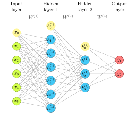
The network diagram
I'm repeating the network diagram from an earlier article as a convenient reference.
What learning is about
The numbers I've used in the earlier article were just a prop to illustrate the mechanism, the out-of-context numbers that lead to meaningless outputs. The goal of the learning process is to find the values of weight matrices and bias vectors so that the network gives "good" outputs for the inputs it has never seen.
There is a really important point that you should never forget: don't hope to reach the "perfect" weights. No matter what machine learning method we choose, no matter what software we use to implement it, and no matter what domain we apply it on, we are not going to make the oracle that always gives the perfect answer. Nor is such answer possible in many cases, since these methods are often use to model non-deterministic things.
Another reason that we can't hope to find perfect coefficients is that the search space is intractably large.
Even a small matrix between a 10-neuron layer and a 30 neuron layer has 300 entries. Even if the weights
were binary, 0 or 1 valued, there would be \(2^{300}\) possible combinations. That is a large number of
combinations to try. But the weights are floating point numbers, so the scope is even larger.
What we can hope, is to find the weights that are good enough. We can not explore each combination, but, luckily, most combinations would be equally bad, so most methods are based on trying only the combinations that have some sense, and then going in the directions that look promising.
Supervised learning and gradient descent
The type of learning that we are using here is called supervised learning. Supervised leaning algorithms work by showing the network the examples of data (inputs) and labels (desired outputs), and adjusting network weights and biases so that the network approximates the outputs for these inputs. This iterative process is called training. If the data examples used in the training represent general data well, we hope that the network will we able to correctly approximate even the instances that it has never seen.
But, how exactly do we adjust the weights? Surely not by blindly trying every possible combination; that is intractable. The most common method for teaching neural networks is gradient descent.
We begin by choosing weight values, usually at random, taking one example from the training data \(x\) and calculating the network output \(a\). Since the weights are random, the output will typically be far away from the result \(y\) from the training data. If we pick some function that can nicely measure that distance, we will be able to tell how far away these two values are. In deep learning terminology, this function is called the cost function (also called the loss function, and sometimes the objective function).
\(C(w,b) \equiv \frac{1}{2n} \sum_x \lVert \mathbf{y}_x - \mathbf{a}_x \lVert ^2\)
We calculate the distance between network outputs and expected outputs for each training example \(x\), average it, and get the number that measures the loss. This particular function is also called quadratic cost, or mean squared error.
So, we know the right answer \(y = f(x)\), we initialized the network weights so that it calculates \(a = g(x)\), we can measure the distance between \(a\) and \(y\), and would like to change weights so that \(a\) becomes as close as possible to \(y\) on average.
In other words, we want to minimize the cost function. This is nice, since instead of "learning", an abstract and magical concept, we are talking about optimization, a subject that is rather well defined and has a clear mathematical background.
Some optimization problems can be solved analytically with precision, some can be explicitly approximated within error range, but neural networks are too large for that. For example, minimum(s) of a function can be found by finding where the first derivative of the function is zero. But, given the size of neural networks, solving that is intractable. The methods that work with more complex problems are usually iterative. They explore the space step by step, in each iteration taking some direction that, hopefully, leads to better solutions. What we usually can't say with these methods is whether we reached the best solution.
Gradient descent is a method that, at each step, takes the direction down the steepest slope. That direction is pointed out by the first derivative of the function. The first derivative of a function defines the rate of change of the function at a particular point. Explaining this background in detail is out of scope of this article, but if you need some, look for some nice text on calculus.
Here is a simplified depiction of gradient descent with a scalar function.
Note that it didn't find the global minimum to the left, but a local one closer to the starting point. There are ways to make this exploration more robust, but there is no way to guarantee the discovery of the global minimum. Luckily, it turns out to not be such a big problem in neural networks. Modern implementations are good enough.
Since we are dealing with vectors, instead of scalars, we use gradient, which is a vector of partial derivatives of C, practically a kind of "vector derivative".
\(\nabla{C} \equiv (\frac{\partial{C}}{\partial{w_1}},\frac{\partial{C}}{\partial{w_2}},\dots)\)
So, we start from a point, move by \(\Delta{C}\approx \nabla{C}\Delta{w}\), and we want to make sure that we are going down (\(\Delta{C}\) is negative), taking the best route \(\Delta{w}\). I'll spare you from the details (explore that in the recommended literature), but it can be shown that the best route is \(\Delta{w} = -\eta\nabla{C}\), which ensures that \(\Delta{C}\approx -\eta\nabla{C}\nabla{C} = -\eta \nabla{C}^2 \leq 0\). Since \(\Delta{C} \leq 0\), the algorithm is guaranteed to go in a good direction.
The size of the step we take, \(\eta\), is called the learning rate. Choosing a good learning rate is important. The gradient only shows the best direction at infinitely small distanc.e The larger the step, the greater the chance that the gradient at that distance changes. Imagine descending from a peak of the mountain and trying to reach the valley. If we make superhuman jumps, we will jump over the valley and land on another peak. If the step is too small, we would need too many steps to reach the bottom of the valley. As many other things in deep learning such as deciding on the structure of the network, it is a craft rather than science. We don't have a formula, and rely on experience, trial, and error.
Backpropagation
We just take the gradient, plug it into the formula \(w' = w + \Delta{w}\) and in a number of iterations, we train the network. Great! But, now we have another problem: how to calculate the gradient?
You've probably heard about automatic differentiation, so we should certainly invoke some magic from an automatic differentiation software package? Not at all. First, these packages are not as powerful as you might imagine. Second, we don't need that sort of magic.
I've already mentioned that the biggest strength of neural networks is in their simple structure. We have a cascade of linear transformations followed by simple activation functions, which have been chosen by design to have very straightforward derivatives. We can easily calculate the gradient of each of these elements in isolation. The trick that's left is how to combine these.
The answer is backpropagation, an algorithm for calculating gradients of each layer by propagating the error backwards, iteratively updating weights.
In each iteration, the signal is propagated forwards, just like during the inference that we've implemented in previous articles. The error is calculated, and based on it, going backwards, the gradient for each layer. Along with calculating gradients, we update the weights and biases. Then, the new training example becomes the input, the new forward step takes place, then the new error is calculated etc.
Some code that we'll need later
This article contains too much prose, and too little code, I know. We need an overview of the learning algorithm we're going to implement in the next articles.
We'll also need a few fairly approachable operations that we haven't used before. It might be a good idea to present them here. We'll use them right away in theory, and in the next articles in practice.
(require '[uncomplicate.commons.core :refer [with-release let-release]]
         '[uncomplicate.neanderthal
           [core :refer [transfer raw copy]]
           [native :refer [dge dv]]
           [vect-math :refer [mul mul! exp tanh! linear-frac! sin cos exp!]]])
The Haddamard product
The Haddamard product of two vectors, \(\mathbf{x} \odot \mathbf{y}\), is a vector that contains products of respective pairs of entries from \(x\) and \(y\).
In Neanderthal, you can compute this vectorized * function by using the mul or mul! function from the
vect-math namespace. That namespace contains vectorized equivalents of the
scalar-based mathematical functions from the math namespace, applied element-wise.
(with-release [x (dv 1 2 3)
               y (dv 4 5 6)]
  (mul x y))
nil#RealBlockVector[double, n:3, offset: 0, stride:1]
[   4.00   10.00   18.00 ]
The destructive variant puts the result into the first vector.
(with-release [x (dv 1 2 3)
               y (dv 4 5 6)]
  (mul! x y)
  (transfer x))
nil#RealBlockVector[double, n:3, offset: 0, stride:1]
[   4.00   10.00   18.00 ]
All functions from the vect-math namespace equally support vectors and matrices.
(with-release [a (dge 2 3 [1 2 3 4 5 6])
               b (dge 2 3 [7 8 9 10 11 12])]
  (mul a b))
nil#RealGEMatrix[double, mxn:2x3, layout:column, offset:0]
   ▥       ↓       ↓       ↓       ┓
   →       7.00   27.00   55.00
   →      16.00   40.00   72.00
   ┗                               ┛
The derivative of a function
Not all functions have derivatives in the whole domain. When there is a derivative, it doesn't mean that it's easy to compute or represent analytically. But, some well-known functions are well known exactly because they have an elegant derivative everywhere.
The finest example is the exponent function. The derivative of the exp function is the
exp function itself! When we have a vector x, computing (exp x) gives us both
the value of the function and the value of the derivative of the function at these points.
(def x (dv 0 0.5 0.7 1))
(exp x)
nil#RealBlockVector[double, n:4, offset: 0, stride:1]
[   1.00    1.65    2.01    2.72 ]
Some other functions are finely paired as a function and its derivative in the simplest expressions.
For example, sin and cos. The derivative of sin is cos, and the derivative of cos is -sin.
In this example, to compute the values of the function sin at each point in the vector x, we invoke
the sin function.
(sin x)
nil#RealBlockVector[double, n:4, offset: 0, stride:1]
[   0.00    0.48    0.64    0.84 ]
To compute the derivative of the sin function at these same points, we invoke the cos function
at these same points.
(cos x)
nil#RealBlockVector[double, n:4, offset: 0, stride:1]
[   1.00    0.88    0.76    0.54 ]
Some well-known functions have analytical derivatives, although they are not that obvious, and a bit harder to compute. One example is the sigmoid function, which is commonly used as an activation function in neural networks.
\begin{equation} \sigma(x) = \frac{1}{1 + e^{-x}} = \frac{e^x}{e^{x} + 1} \end{equation}Fortunately, the sigmoid function has a nice formula for the derivative. Here it is:
\begin{equation} \sigma ' = \frac{d\sigma}{d{x}} = \sigma(x) \dot (1 - \sigma(x)) \end{equation}We have already implemented the sigmoid function.
(defn sigmoid! [x]
  (linear-frac! 0.5 (tanh! (linear-frac! 0.5 x 0.0)) 0.5))
Now, since we have the sigmoid function, it should be easy to implement its derivative.
We just invoke a haddamard product on a sigmoid, and a sigmoid subtracted from one.
The logic is easy, but the implementation is not so straightforward. We can easily compute (sigmoid! x).
We can also easily subtract that result from the 1-vector using linear-frac!. However, for the Haddamard
product, we need both of these intermediate results that reside in the same memory for the multiplication.
We can't have them at the same time, and we need a "working" memory.
We could create it internally
each time the function is invoked, and release it after the function is evaluated. This is a clean
solution, but wasteful, considering that we will call this function many times in the learning process.
Another solution is to provide this working space as an additional argument. Here, I design
sigmoid-prim to return both the sigmoid (x!) and its derivative (prim!).
(defn sigmoid-prim!
  ([x!]
   (with-release [x-raw (raw x!)]
     (sigmoid-prim! x! x-raw)))
  ([x! prim!]
   (let [x (sigmoid! x!)]
     (mul! (linear-frac! -1.0 x 1.0 prim!) x))))
Now, given a vector x, we can compute both the value of sigmoid, and its derivative at x.
(let [x (dv 0.1 0.5 0.9 (/ Math/PI 2.0))]
 [(transfer x) (sigmoid-prim! x)])
nil[#RealBlockVector[double, n:4, offset: 0, stride:1]
[   0.10    0.50    0.90    1.57 ]
 #RealBlockVector[double, n:4, offset: 0, stride:1]
[   0.00    0.24    0.21    0.14 ]
]
The four important equations
Now, we can return to the key functions for implementing backpropagation-based gradient descent in neural networks.
You can look for the details in Michael's book; here I summarize the equations that we're going to base our implementation on.
The forward pass
We have already implemented this as part of the inference calculation, but I repeat it here for reference.
\(a^l = \sigma(w^l a^{l-1} + b^l)\)
This equation says that the activated output \(a\) in each layer \(l\) is calculated by calling the activation function \(\sigma\) on the output of the product of weights at that layer \(w^l\) and the output of the previous layer, \(a^{l-1}\), increased by bias \(b^l\). The input to \(\sigma\) will be useful during the backpropagation, so we can keep it as \(z\), and the equation becomes:
\(a^l = \sigma(z^l)\), where \(z^l = w^l a^{l-1} + b^l\).
Please note that σ here stands for any activation function, not only the sigmoid function.
The error of the output layer δL (1)
The error of the output layer can be computed as a haddamard product of the gradient of the cost function in respect to the activation \(a\) and the derivative of \(z\).
\(\delta^L = \nabla_a C \odot \sigma ' (z^L)\)
The exact formula for \(\nabla_a C\) depends on which cost function we choose. For the quadratic cost function, that gradient will be as simple as \(a^L - y\).
\(\delta^L = (a^L - y) \odot \sigma ' (z^L)\)
The error of hidden layers δl (2)
The error in hidden layers is generic. It depends only on the weights and the error of the next layer, and the derivative of its own pre-activation outputs.
\(\delta^l = ((w^{l+1})^T \delta^{l+1}) \odot \sigma ' (z^L)\)
The rate of change of the cost in respect to bias (3)
Gradient in respect to biases in each layer is equal to the error we have computed.
\(\nabla_b C^l = \delta^l\)
The rate of change of the cost in respect to weights (4)
Gradient in respect to weights depends on the error of that layer and the activations of the previous layer
\(\nabla_w C^l = a^{l-1} \delta^l\)
From these equations, we can see that during the backpropagation, in each layer, we need some data from the next layer, and some data from the previous layer. This have two major consequences. The first is that, when building the network, we have to decide on how to connect this chain, which is not trivial since the dependencies between layers go in both directions. The second is that, should we decide to optimize the memory consumption and reuse some memory, we need to be careful, since some data might be needed more than once during the forward and backward passes.
The next article
In the next articles, we take these four fundamental equations, and implement the algorithm step by step, taking care of the performance and discussing the implications of each step.
Thank you
Clojurists Together financially supported writing this series. Big thanks to all Clojurians who contribute, and thank you for reading and discussing this series.