Deep Learning from Scratch to GPU - 6 - CUDA and OpenCL
February 28, 2019
Please share this post in your communities. Without your help, it will stay burried under tons of corporate-pushed, AI and blog farm generated slop, and very few people will know that this exists.
These books fund my work! Please check them out.
If you haven't yet, read my introduction to this series in Deep Learning in Clojure from Scratch to GPU - Part 0 - Why Bother?.
The previous article, Part 5, is here: Sharing Memory.
To run the code, you need a Clojure project with Neanderthal () included as a dependency. If you're in a hurry, you can clone Neanderthal Hello World project.
Don't forget to read at least some introduction from Neural Networks and Deep Learning, start up the REPL from your favorite Clojure development environment, and let's continue with the tutorial.
(require '[uncomplicate.commons.core :refer [with-release let-release Releaseable release]]
         '[uncomplicate.clojurecuda.core :as cuda :refer [current-context default-stream synchronize!]]
         '[uncomplicate.clojurecl.core :as opencl :refer [*context* *command-queue* finish!]]
         '[uncomplicate.neanderthal
           [core :refer [axpy! scal! transfer! transfer mm! rk! view-ge vctr ge entry!]]
           [native :refer [native-double native-float dv dge]]
           [vect-math :refer [tanh! linear-frac!]]
           [cuda :refer [cuda-float]]
           [opencl :refer [opencl-float]]])
(import 'clojure.lang.IFn)
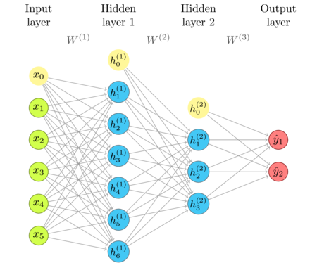
The network diagram
I'm repeating the network diagram from the previous article as a convenient reference.

The inference layer type
We're starting from the existing layer type, and trim it down a bit. The single-input function is redundant. We keep just the batch version.
(defprotocol Parameters
  (weights [this])
  (bias [this]))

(deftype FullyConnectedInference [w b activ-fn]
  Releaseable
  (release [_]
    (release w)
    (release b))
  Parameters
  (weights [this] w)
  (bias [this] b)
  IFn
  (invoke [_ x ones a]
    (activ-fn (rk! -1.0 b ones (mm! 1.0 w x 0.0 a)))))
All functions that we have used, axpy, mm, etc., are polymorphic and general
in respect to the device they execute on: CPU, Nvidia GPU, AMD GPU, and Intel GPU.
The activation functions that we have used are general, too.
(defn sigmoid! [x]
  (linear-frac! 0.5 (tanh! (scal! 0.5 x)) 0.5))
The dispatch to the right implementation is being done by the type of the vector or matrix structure
at hand. The constructor function that we have used is hard-coded for using double floating point numbers,
to exist in main memory, and use the native CPU backend (dge and dv constructors).
(defn fully-connected [activ-fn in-dim out-dim]
  (let-release [w (dge out-dim in-dim)
                bias (dv out-dim)]
    (->FullyConnectedInference w bias activ-fn)))
Generalize the code
There is only one thing that we have to do to make this code completely general:
use general constructors from the core namespace, instead of the convenience methods from
the native namespace. These methods are, in this case, ge (general matrix) instead of
dge (double general native matrix), and vctr instead of dv (double native vector).
The only difference in these methods is that they require an engine-specific factory
as their first argument. We accommodate the fully-connected constructor to accept it as
an input.
(defn fully-connected [factory activ-fn in-dim out-dim]
  (let-release [w (ge factory out-dim in-dim)
                bias (vctr factory out-dim)]
    (->FullyConnectedInference w bias activ-fn)))
Now, we repeat the example of running the network with native-double. That is the same factory
that is used by the dge and dv methods, available in the native namespace. We can use
native-float in its place, to use single-precision floating point computations on the CPU,
or some of the GPU factories, or configure another factory coded by a 3-rd party, or even
use the same code provided by Neanderthal, but configured in a different way.
(with-release [x (ge native-double 2 2 [0.3 0.9 0.3 0.9])
               ones (vctr native-double 1 1)
               layer-1 (fully-connected native-double tanh! 2 4)
               a-1 (ge native-double 4 2)
               layer-2 (fully-connected native-double sigmoid! 4 1)
               a-2 (ge native-double 1 2)]
  (transfer! [0.3 0.1 0.9 0.0 0.6 2.0 3.7 1.0] (weights layer-1))
  (transfer! [0.7 0.2 1.1 2] (bias layer-1))
  (transfer! [0.75 0.15 0.22 0.33] (weights layer-2))
  (transfer! [0.3] (bias layer-2))
  (transfer (layer-2 (layer-1 x ones a-1) ones a-2)))
nil#RealGEMatrix[double, mxn:1x2, layout:column, offset:0]
   ▥       ↓       ↓       ┓
   →       0.44    0.44
   ┗                       ┛
I modified the result display of this example a bit. Instead of doing a println as in the previous
articles, I transfer the resulting matrix to main-memory. I do it for convenience, since this blog
post and its results are automatically generated from live code, and also to teach a few patterns in
this type of coding.
Don't forget that, in this example, I have used with-release for all bindings, even the output
a-2. I do this because the code should support CPU and GPU. On the CPU, releasing the data
is of great help, but is optional in a REPL session, since the memory eventually gets released by the JVM
(with a few caveats since JVM might not do it as soon as you hoped). On the GPU, however, JVM can not do anything;
the underlying GPU buffer that is not released explicitly, is not released at all until we release the whole context.
Therefore, the habit that I recommend, is to always take care of that and release all vectors, matrices
and other structures as soon as possible.
However, we'd like to see the result in the REPL. But, how, if the data stored in the result that
is being returned (a-2) is released just the moment before it needs to be printed. Here, the transfer method
transfers the data from wherever it is (main memory or GPU memory) to the equivalent object in the main memory.
This particular network
We are going to run this code on different devices, and I think it is a good idea to
wrap it into a function. Note that we provide factory as the argument, and everything else is
general and the same for all platforms!
(defn this-particular-network [factory]
  (with-release [x (ge factory 2 2 [0.3 0.9 0.3 0.9])
                 ones (vctr factory 1 1)
                 layer-1 (fully-connected factory tanh! 2 4)
                 a-1 (ge factory 4 2)
                 layer-2 (fully-connected factory sigmoid! 4 1)
                 a-2 (ge factory 1 2)]
    (transfer! [0.3 0.1 0.9 0.0 0.6 2.0 3.7 1.0] (weights layer-1))
    (transfer! [0.7 0.2 1.1 2] (bias layer-1))
    (transfer! [0.75 0.15 0.22 0.33] (weights layer-2))
    (transfer! [0.3] (bias layer-2))
    (transfer (layer-2 (layer-1 x ones a-1) ones a-2))))
I can call this function and instruct it to use double-precision floating point computation on the CPU.
(this-particular-network native-double)
nil#RealGEMatrix[double, mxn:1x2, layout:column, offset:0]
   ▥       ↓       ↓       ┓
   →       0.44    0.44
   ┗                       ┛
Or, it can use single-precision floating point computation, still on the CPU.
(this-particular-network native-float)
nil#RealGEMatrix[float, mxn:1x2, layout:column, offset:0]
   ▥       ↓       ↓       ┓
   →       0.44    0.44
   ┗                       ┛
With CUDA on an Nvidia GPU
The same code, without changes, runs on the GPU! The only thing that it needs, is the factory that sets it up with appropriate engines.
For engines based on Nvidia's CUDA platform, we use the functions from
uncomplicate.clojurecuda.core namespace to choose and set up the GPU itself.
We may have more than one graphics accelerator in our system, and Neanderthal
has to know which one to use. with-default is a method that will choose the best
device that you have, and set it up automatically. There are more fine grained
methods in the ClojureCUDA () library if you need more control.
Next, we use the cuda-float constructor to create a factory whose engines will use
single-precision floating point computations in the default context and stream provided by
ClojureCUDA. We may need more than one factory for advanced computations.
(cuda/with-default
  (with-release [cuda-factory (cuda-float (current-context) default-stream)]
    (this-particular-network cuda-factory)))
nil#RealGEMatrix[float, mxn:1x2, layout:column, offset:0]
   ▥       ↓       ↓       ┓
   →       0.44    0.44
   ┗                       ┛
With OpenCL on an AMD GPU
In case you have an AMD or Intel GPU, you won't be able to work with CUDA platform. Don't worry, Neanderthal supports OpenCL, which is an open platform equivalent to CUDA, that supports all major hardware vendors: AMD, Intel, and even Nvidia.
Instead of ClojureCUDA, you'll use ClojureCL () to set up your execution environment. Other than a few differences in terminology, most of the knowledge of parallel computing on the GPU is transferable between CUDA and OpenCL.
(opencl/with-default
  (with-release [opencl-factory (opencl-float *context* *command-queue*)]
    (this-particular-network opencl-factory)))
nil#RealGEMatrix[float, mxn:1x2, layout:column, offset:0]
   ▥       ↓       ↓       ┓
   →       0.44    0.44
   ┗                       ┛
You can even mix CUDA and OpenCL
With Neanderthal, you can even combine code that partly runs on a Nvidia GPU and partly on an AMD GPU. For performance reasons, I can not imagine why you'd want to do this. Don't do it in "real" code. But, do it for fun and learning. I included this example only to show you how flexible Neanderthal and Clojure are. This is something that you'd struggle to do in competing platforms, if at all!
(opencl/with-default
  (cuda/with-default
      (with-release [opencl-factory (opencl-float *context* *command-queue*)
                     cuda-factory (cuda-float (current-context) default-stream)
                     x (ge opencl-factory 2 2 [0.3 0.9 0.3 0.9])
                     ones-opencl (vctr opencl-factory 1 1)
                     layer-1 (fully-connected opencl-factory tanh! 2 4)
                     a-1 (ge opencl-factory 4 2)
                     a-1-cuda (ge cuda-factory 4 2)
                     ones-cuda (vctr cuda-factory 1 1)
                     layer-2 (fully-connected cuda-factory sigmoid! 4 1)
                     a-2 (ge cuda-factory 1 2)]
        (transfer! [0.3 0.1 0.9 0.0 0.6 2.0 3.7 1.0] (weights layer-1))
        (transfer! [0.7 0.2 1.1 2] (bias layer-1))
        (transfer! [0.75 0.15 0.22 0.33] (weights layer-2))
        (transfer! [0.3] (bias layer-2))
        (layer-1 x ones-opencl a-1)
        (transfer! a-1 a-1-cuda)
        (transfer (layer-2 a-1-cuda ones-cuda a-2)))))
nil#RealGEMatrix[float, mxn:1x2, layout:column, offset:0]
   ▥       ↓       ↓       ┓
   →       0.44    0.44
   ┗                       ┛
Micro benchmark
One aspect of GPU computing is how to do it at all. As I hope you'd agree, with Neanderthal, ClojureCL and ClojureCUDA it is not that hard. Another question is: is it worth the trouble?
Nvidia GTX 1080 Ti (2017)
I'll measure the same superficial example that we used in the last post. The heavily-optimized native CPU engine backed by Intel's MKL (the fastest CPU thing around) computed one pass in 6 seconds. We hope that Nvidia's GeForce GTX 1080Ti (11 TFLOPS) will be able to do it in much less time.
Please note the (synchronize!) call; GPU calls are asynchronous, and here we are making sure
that we block the main thread and wait for the computation to complete before we declare victory.
(cuda/with-default
  (with-release [factory (cuda-float (current-context) default-stream)]
    (with-release [x (ge factory 10000 10000)
               ones (entry! (vctr factory 10000) 1)
               layer-1 (fully-connected factory tanh! 10000 5000)
               a1 (ge factory 5000 10000)
               layer-2 (fully-connected factory sigmoid! 5000 1000)
               a2 (ge factory 1000 10000)
               layer-3 (fully-connected factory sigmoid! 1000 10)
               a3 (ge factory 10 10000)]
      (time
       (do
         (layer-3 (layer-2 (layer-1 x ones a1) ones a2) ones a3)
         (synchronize!))))))
niltrue
"Elapsed time: 122.529925 msecs"
And it does! 122 milliseconds. This is roughly 50 times faster than the optimized engine on my CPU!
AMD R9 290X (2013)
In my system, I also have an old-ish AMD GPU, R9 290X, a beast in its days at 5 TFLOPS.
(opencl/with-default
  (with-release [factory (opencl-float *context* *command-queue*)]
    (with-release [x (ge factory 10000 10000)
               ones (entry! (vctr factory 10000) 1)
               layer-1 (fully-connected factory tanh! 10000 5000)
               a1 (ge factory 5000 10000)
               layer-2 (fully-connected factory sigmoid! 5000 1000)
               a2 (ge factory 1000 10000)
               layer-3 (fully-connected factory sigmoid! 1000 10)
               a3 (ge factory 10 10000)]
      (layer-1 x ones a1) ;; The first time a BLAS operation is used in OpenCL might incur initialization cost.
      (finish!)
      (time
       (do
         (layer-3 (layer-2 (layer-1 x ones a1) ones a2) ones a3)
         (finish!))))))
"Elapsed time: 330.683851 msecs"
Roughly 3 times slower than Nvidia. Still worth it, since it is almost 20 times faster than the CPU.
You may expect it to be closer to Nvidia's result, since it should be twice as slow by the specifications (5 TFOPS vs 11 TFLOPS). Instead of Nvidia's proprietary BLAS matrix routines, Neanderthal uses an open-source engine in its OpenCL backend. Although it's not that much behind, it can not match Nvidia's hardware optimization at the same level. If you have an Nvidia's GPU, you can use ClojureCL (), but if you need maximum performance, use ClojureCUDA ().
Performance comparison (in this case)
Let me sum it up. In this example, we managed to accelerate a top-performance CPU code by 20 times with an old AMD GPU, and 50 times with a fairly recent but not the best Nvidia GPU, keeping the same code!
Donations
While you're still in amazement, let me sneak in a quick reminder that I'm accepting donations that I hope will support the development of these cool Clojure libraries in the years to come.
If you feel that you can afford to help, and wish to donate, I even created a special Starbucks for two tier at patreon.com/draganrocks, for the generous readers of this article. Don't worry, I won't squander the donations at Starbucks. But, not because I don't like a good mocha! There's no Starbucks shops in my country, that's all. If you feel specially generous, you can do something even cooler: adopt a pet function.
The next article
We started with 180 seconds, made it faster by 30 times by introducing batches, and even further, by 50 times by running it on the GPU. This is 1500 times faster than looping the single-input pass, which is itself optimized by MKL (and not using any naive code). But, hey, 180 seconds is not that long. Why bother with GPU instead of waiting these measly 3 minutes? Yes, 3 minutes might be tolerable in many cases. Before the Starbucks barista even gets to adding cream on top of that tasty sugar bomb I'm waiting for, voila, the results are ready.
However, during the inference we only do one forward pass through the network. To discover the weights, that is, to learn the network, we need a forward and a backward pass, and then repeat that many, many times. At least a few dozen, but may be hundreds or thousands of times. In that case, 1500 times faster might mean waiting one minute instead of the whole day (1440 minutes)! Now, that is worth the effort in my book.
Finally, we can direct our attention to that challenge: learning the network weights. The next article will be Learning and Backpropagation.
Thank you
Clojurists Together financially supported writing this series. Big thanks to all Clojurians who contribute, and thank you for reading and discussing this series.

