Deep Learning from Scratch to GPU - 8 - The Forward Pass (CUDA, OpenCL, Nvidia, AMD, Intel)
March 13, 2019
Please share this post in your communities. Without your help, it will stay burried under tons of corporate-pushed, AI and blog farm generated slop, and very few people will know that this exists.
These books fund my work! Please check them out.
We start implementing stochastic gradient descent and the backpropagation algorithm. Here we implement the forward pass of the training layer and run it on the CPU and GPU.
If you haven't yet, read my introduction to this series in Deep Learning in Clojure from Scratch to GPU - Part 0 - Why Bother?.
The previous article, Part 7, is here: Learning and Backpropagation.
To run the code, you need a Clojure project with Neanderthal () included as a dependency. If you're in a hurry, you can clone Neanderthal Hello World project.
Don't forget to read at least some introduction from Neural Networks and Deep Learning, start up the REPL from your favorite Clojure development environment, and let's continue with the tutorial.
(require '[uncomplicate.commons.core
           :refer [with-release let-release Releaseable release]]
         '[uncomplicate.clojurecuda.core :as cuda
           :refer [current-context default-stream synchronize!]]
         '[uncomplicate.clojurecl.core :as opencl
           :refer [*context* *command-queue* finish!]]
         '[uncomplicate.neanderthal
           [core :refer [mrows dim raw view axpy! copy! scal! transfer!
                         transfer mm! rk! view-ge vctr ge entry!]]
           [native :refer [native-float]]
           [vect-math :refer [tanh! linear-frac!]]
           [cuda :refer [cuda-float]]
           [opencl :refer [opencl-float]]])
(import 'clojure.lang.IFn)
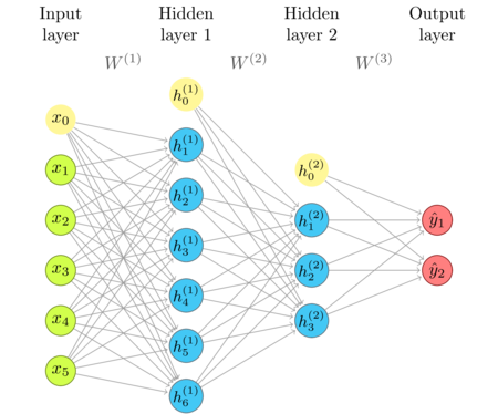
The network diagram
I'm repeating the network diagram from the previous article as a convenient reference.

The relevant equations
The layer itself computes the linear transformation \(z^l\), and its non-linear activation \(a^l\).
\(a^l = \sigma(z^l)\), where \(z^l = w^l a^{l-1} + b^l\).
Then, in the backward pass, we need the result of the linear transformation \(z^l\) to compute the updates.
In the output layer:
\(\delta^L = \nabla_a C \odot \sigma ' (z^L)\).
In other layers:
\(\delta^l = ((w^{l+1})^T \delta^{l+1}) \odot \sigma ' (z^L)\).
Note that in both of these formulas, we compute the Haddamard product of a matrix that comes from the next layer (\(\nabla_a C\) and \((w^{l+1})^T \delta^{l+1}\)) and the matrix that is located in the layer at hand (\(\sigma ' (z^L)\)).
The inference layer
The existing layer type performs all computations that we need for the forward pass. However, it does not remember data that will be useful in the backward pass. Let's examine it and see what we need to fix.
(defprotocol Parameters
  (weights [this])
  (bias [this]))

(defprotocol ActivationProvider
  (activation-fn [this]))
(deftype FullyConnectedInference [w b activ-fn]
  Releaseable
  (release [_]
    (release w)
    (release b))
  Parameters
  (weights [_] w)
  (bias [_] b)
  ActivationProvider
  (activation-fn [_] activ-fn)
  IFn
  (invoke [_ x ones a]
    (activ-fn (rk! -1.0 b ones (mm! 1.0 w x 0.0 a)))))
Instead of keeping \(z^l\) around, we overwrite it by using a for both the linear output
and, later, the activation.
(defn fully-connected [factory activ-fn in-dim out-dim]
  (let-release [w (ge factory out-dim in-dim)
                bias (vctr factory out-dim)]
    (->FullyConnectedInference w bias activ-fn)))
The training layer
In the inference layer, we didn't have a need for outputs once the signal passes the layer. Now, we do. First, we need to keep \(z^l\) around. As the relevant equations suggest, we also need access to the output of the previous layer, \(a^{l-1}\), and the error propagated from the subsequent layers.
We will work out the details in the following articles, but, for now,
we can see that each training layer should have its own reference to z.
We create the Backprop protocol with methods for moving forward and backward,
and for accessing the activation. Since, by design, all layers in the network operate on
the same batch size, we can reuse the vector of ones by propagating it from each layer to the next
during the construction.
(defprotocol Backprop
  (forward [this])
  (backward [this]))
(defprotocol Transfer
  (input [this])
  (output [this])
  (ones [this]))
The major novelty in FullyConnectedTraining is how we treat the input and output matrices.
In the inference layer implementation, these were function arguments unrelated to the layer
object. In the training layer, they become part of the layer.
Instead of implementing invoke, we implement forward, while most other differences
are related to bookkeeping.
(deftype FullyConnectedTraining [w b a-1 z a ones-vctr activ-fn]
  Releaseable
  (release [_]
    (release w)
    (release b)
    (release a-1)
    (release z)
    (release a)
    (release ones))
  Parameters
  (weights [_] w)
  (bias [_] b)
  Transfer
  (input [_] a-1)
  (output [_] a)
  (ones [_] ones-vctr)
  Backprop
  (forward [_]
    (activ-fn (rk! -1.0 b ones-vctr (mm! 1.0 w a-1 0.0 z)) a))
  (backward [_]
    (throw (ex-info "TODO"))))
The activation function is not allowed to overwrite the argument, so we
create a two-argument version. The input x (z) is unchanged, while the output y (a)
is overwritten with the result.
(defn sigmoid!
  ([x]
   (linear-frac! 0.5 (tanh! (scal! 0.5 x)) 0.5))
  ([x y]
   (linear-frac! 0.5 (tanh! (scal! 0.5 (copy! x y))) 0.5)))
Constructors have some interesting details. I decided that the training layer is going to be wrapped around an inference layer, a sort of an "attachment" to it. Once the training layer trains the parameters, we can dispose it, and continue using the lighter inference layer, without it knowing how these weights and biases were determined.
(defn training-layer
  ([inference-layer input ones-vctr]
   (let-release [w (view (weights inference-layer))
                 b (view (bias inference-layer))
                 a-1 (view input)
                 z (ge w (mrows w) (dim ones-vctr))
                 a (raw z)
                 o (view ones-vctr)]
     (->FullyConnectedTraining w b a-1 z a o (activation-fn inference-layer))))
  ([inference-layer previous-backprop]
   (training-layer inference-layer
                   (output previous-backprop)
                   (ones previous-backprop))))
w and b are just views of the same underlying memory from the inference layer.
view is a polymorphic Neanderthal function that creates a default Neanderthal structure
that reuses the underlying memory of the argument. In this case, we use it to create
additional instances of matrices, that operate on the same data, while having a separate life-cycle.
Releasing views does not release the buffers in the "master" structure.
The reference a-1 is a view that can read and write data from a of the previous
layer, but when we release a-1, that does not affect the previous layer. Of course, if we released
the previous layer, the layer at hand will raise an error if we tried to use its a-1.
z and a are master properties of this layer. They have the same dimensions. ones is also a view.
Creating and using the layers
We are still using the low-level API that directly creates layers. Continuing with the same example from the previous articles, we create two inference layers, but now we create training layers for each. Instead of invoking inference layers as functions, now we invoke the forward method on training layers. At the end, we read the output from the last layer's activation.
(with-release [x (ge native-float 2 2 [0.3 0.9 0.3 0.9])
               ones (vctr native-float 1 1)
               layer-1 (fully-connected native-float tanh! 2 4)
               layer-2 (fully-connected native-float sigmoid! 4 1)
               training-layer-1 (training-layer layer-1 x ones)
               training-layer-2 (training-layer layer-2 training-layer-1)]
  (transfer! [0.3 0.1 0.9 0.0 0.6 2.0 3.7 1.0] (weights layer-1))
  (transfer! [0.7 0.2 1.1 2] (bias layer-1))
  (transfer! [0.75 0.15 0.22 0.33] (weights layer-2))
  (transfer! [0.3] (bias layer-2))
  (forward training-layer-1)
  (forward training-layer-2)
  (transfer (output training-layer-2)))
nil#RealGEMatrix[float, mxn:1x2, layout:column, offset:0]
   ▥       ↓       ↓       ┓
   →       0.44    0.44
   ┗                       ┛
Hey, this is the same result as before. Good job (for now :)
I think it would be a good idea to leave something easy for exercise. Following the earlier article and the upcoming benchmarking code for CUDA and OpenCL, you can test yourself whether this code works correctly on the GPU.
The required memory in training layers increased in regard to plain inference layers.
We now have to keep both z and a, which takes twice the number of neurons in the layer times batch size.
Micro benchmark
Having tested the correctness of what we have implemented in this article, I think it would be a good idea to also test the speed. Does a slight change in having to keep more data around affect the speed of computations?
Nvidia GTX 1080 Ti (2017)
(cuda/with-default
  (with-release [factory (cuda-float (current-context) default-stream)]
    (with-release [x (ge factory 10000 10000)
                   ones (entry! (vctr factory 10000) 1)
                   layer-1 (fully-connected factory tanh! 10000 5000)
                   layer-2 (fully-connected factory sigmoid! 5000 1000)
                   layer-3 (fully-connected factory sigmoid! 1000 10)
                   training-layer-1 (training-layer layer-1 x ones)
                   training-layer-2 (training-layer layer-2 training-layer-1)
                   training-layer-3 (training-layer layer-3 training-layer-2)]
      (time
       (do
         (forward training-layer-1)
         (forward training-layer-2)
         (forward training-layer-3)
         (synchronize!))))))
niltrue
"Elapsed time: 119.121297 msecs"
Saving intermediate results did not increase the running time. That's good news!
AMD R9 290X (2013)
(opencl/with-default
  (with-release [factory (opencl-float *context* *command-queue*)]
    (with-release [x (ge factory 10000 10000)
                   ones (entry! (vctr factory 10000) 1)
                   layer-1 (fully-connected factory tanh! 10000 5000)
                   layer-2 (fully-connected factory sigmoid! 5000 1000)
                   layer-3 (fully-connected factory sigmoid! 1000 10)
                   training-layer-1 (training-layer layer-1 x ones)
                   training-layer-2 (training-layer layer-2 training-layer-1)
                   training-layer-3 (training-layer layer-3 training-layer-2)]
      (forward training-layer-1)
      (finish!)
      (time
       (do
         (forward training-layer-1)
         (forward training-layer-2)
         (forward training-layer-3)
         (finish!))))))
"Elapsed time: 337.34171 msecs"
Compared to 337 ms we got before, we see that there is no slowdown in the OpenCL implementation either.
Donations
If you feel that you can afford to help, and wish to donate, I even created a special Starbucks for two tier at patreon.com/draganrocks. You can do something even cooler: adopt a pet function.
The next article
In the next article, we will see what should be improved in the current implementation to enable the backward pass. As it is easy, we'll continue running everything on CPU, an Nvidia GPU and an AMD GPU.
Thank you
Clojurists Together financially supported writing this series. Big thanks to all Clojurians who contribute, and thank you for reading and discussing this series.

